Getting Started with a simple conditional distribution model -- Python

For further information on theories and implementations, refer to the robotics book: https://www.roboticsbook.org/

In this notebook, we walk through an simple example of:

Representing discrete random variables in gtsam
Building a bayes net with the discrete random variables
Visualizing the bayes net we built
Doing effecient inference with gtsam FactorGraphs (reducing the inference time from exponential to polynomial)!

Other Installs and Imports¶

Some of the visualizations below use graphviz. That is not super easy to install except when using conda, in which case it is a one-liner:

conda install -c conda-forge python-graphviz

It is also installed by default on Colab.

try:
    import google.colab
    %pip install -U -q gtbook # this installs more visualization mojo, but needs graphviz!
except ImportError:
    pass

import gtsam
import gtbook
from gtbook import display

Representing Discrete Random Variables¶

For this simple example, think of a Robot that is moving between different rooms for several seconds. After 1, 2, 3, ... n seconds, the robot wouldn’t be sure where it is any more. So for each timestamp t (1,2,3, ...n), we use a random variable $X_t$ to represent the probability of the robot in each room.

We have only 5 rooms ['Living Room', 'Kitchen', 'Office', 'Hallway', 'Dining Room'] variable X can take on. So each $X_t$ is a probability distribution over these 5 states. Let’s represent that in gtsam.

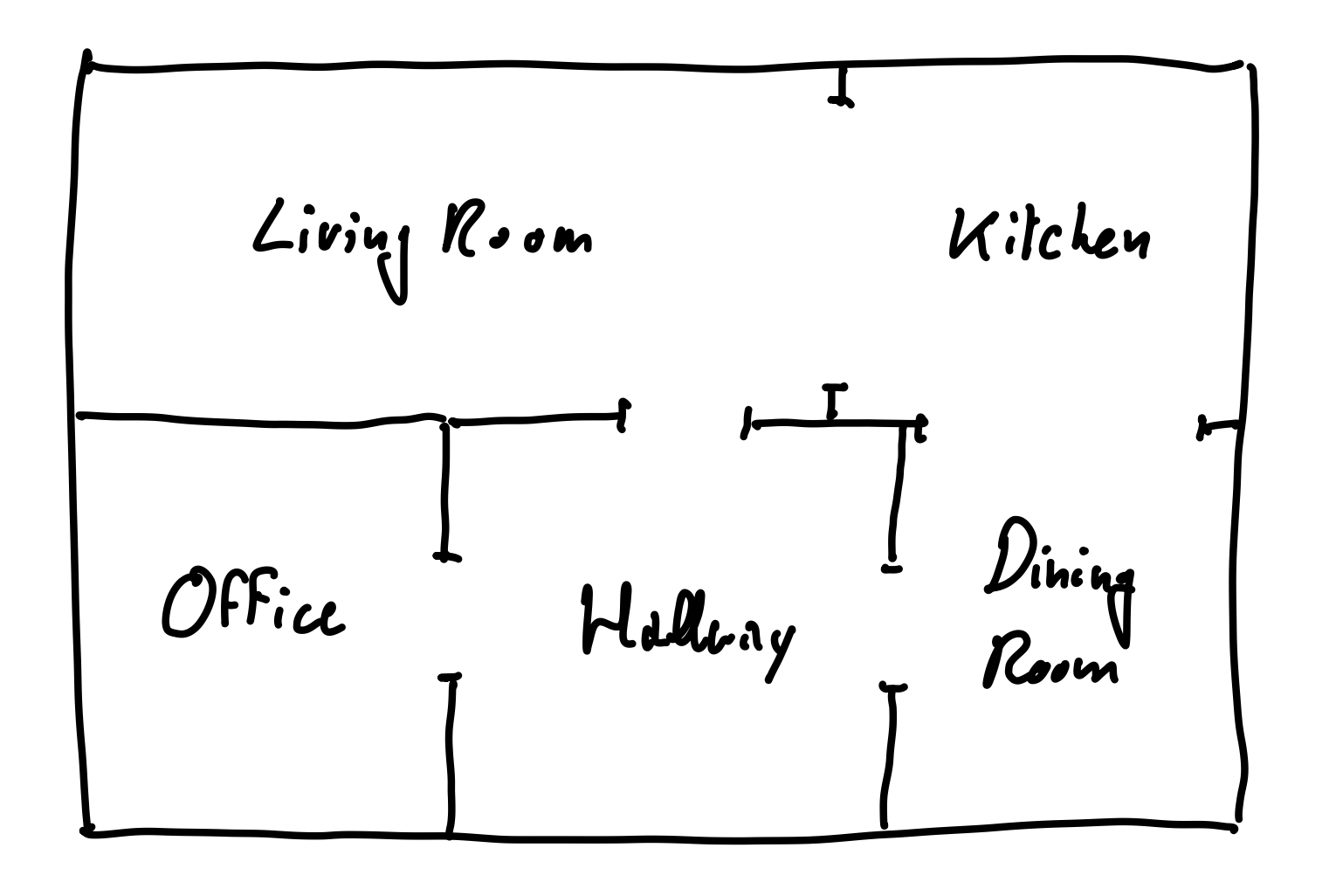
Figure 1:The floor plan of a house in which our hypothetical vacuum cleaning robot will operate.

# We want to create random variables X1, X2, X3, ...
from gtbook.discrete import Variables
VARIABLES = Variables()

# The possible states of the random variable
room_states = ['Living Room', 'Kitchen', 'Office', 'Hallway', 'Dining Room']

# create a discrete variable with states

#                   name,    states
X1 = VARIABLES.discrete('X1', room_states)
X2 = VARIABLES.discrete('X2', room_states)
X3 = VARIABLES.discrete('X3', room_states)
X4 = VARIABLES.discrete('X4', room_states)

print(X1)
print(X4)

(0, 5)
(3, 5)

We have just created random variables $X1, X2, X3, X4$ . Each one is a discrete variable that has probability of being in each of the room_states.

The printed output we see for X1 and X2 is a tuple (key, cardinality). The key is the gtsam internal representation of the variable. Cardinality in our case is just the number of rooms: 5.

At any time, if you are confused about how to use a function or how to interpret the result, you can run

help(VARIABLES.discrete)

Help on method discrete in module gtbook.discrete:

discrete(name: str, domain: list[str]) -> tuple[int, int] method of gtbook.discrete.Variables instance
    Create a variable with given name and discrete domain of named values.

    Args:
        name (str): name of the variable.
        domain (list[str]): names for the different values.

    Returns:
        DiscreteKey, i.e., (gtsam.Key, cardinality)

Discrete Series¶

In the previous example, it’s a bit tedious to create each variable one by one. We can use gtsam.Variables.discrete_series to create a series of discrete variables with the same cardinality.

X = VARIABLES.discrete_series('X', range(1, 5), room_states)
print(X)
print(f"X1: {X[1]}")
print(f"X4: {X[4]}")

{1: (6341068275337658369, 5), 2: (6341068275337658370, 5), 3: (6341068275337658371, 5), 4: (6341068275337658372, 5)}
X1: (6341068275337658369, 5)
X4: (6341068275337658372, 5)

Here, we see the keys got much longer, but the object is really exactly the same as what we had above. For more details on how this value is constructed, see here.

Assigning Probabilities¶

We can now assign probabilities to each variable. Let’s initialize X1 to be in the Living Room with 80% probability, and the rest of the rooms with 5% probability each.

Create a Graph gtsam.DiscreteFactorGraph to record the assignments.
Add the variables to the graph with the assigned probabilities.

Don’t get frustrated by the term FactorGraph, it’s just a graph that holds variables and their probabilities. To learn more about FactorGraphs, and how we use it to perform optimization, view the roboticsbook and the gtsam documentation.

# create graph
graph = gtsam.DiscreteFactorGraph()

# adding probabilities for X1
# X = ['Living Room', 'Kitchen', 'Office', 'Hallway', 'Dining Room']
prob = [0.8, 0.05, 0.05, 0.05, 0.05]  # P(X1)
graph.add(X[1], prob)  # P(X1)

# Let's view the assignments by printing the graph: 

def pretty(obj):
    return gtbook.display.pretty(obj, VARIABLES) # function to display 

pretty(graph)

# This cell won't run if you don't have graphviz installed!
display.show(graph)

# Alternatively, you can also specify the probabilities in string format!
# Plus, they don't have to sum to 1, gtsam will normalize them for you. So you can also give them in terms of frequency

graph2 = gtsam.DiscreteFactorGraph()
# This works:
# graph2.add(X[1], "0.8 0.05 0.05 0.05 0.05")  # P(X1)

# This also works:
graph2.add(X[1], "80 5 5 5 5")  # P(X1) in terms of frequency

pretty(graph2)

Conditional Probability¶

Let’s now move between the rooms! Let’s allow the robot to move up, down, left, right. And after taking each action, the room X the robot is in change. To do this, introduce a new variable $A$ that represent what actions we took, and make next next room the robot with be in $X_{t+1}$ , depend (conditional) on the action it takes $A_t$ , and where it currently is $X_t$ .

Here we focus on building the conditional probability. To learn more about how this simulated robot environment works, visit robotics-book-ch3

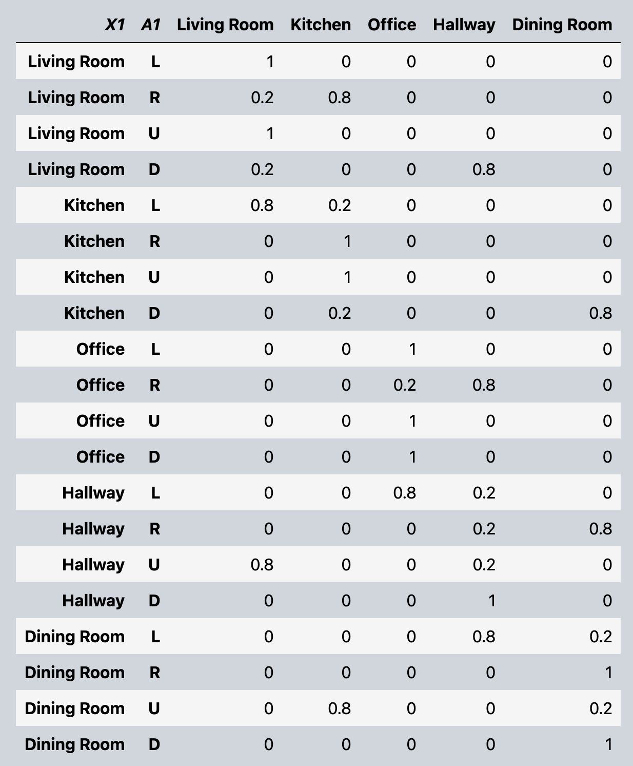
Below is the probability table we want to model. Given, current room X1, action A1, what’s the probability of being in each room in X2.

# Great. Let's now represent 

room_states = ['Living Room', 'Kitchen', 'Office', 'Hallway', 'Dining Room']
action_states = ['L', 'R', 'U', 'D'] # Left, Right, Up, Down
# create a discrete variable with states

#                   name,    states
X = VARIABLES.discrete_series('X', range(1, 5), room_states)
A = VARIABLES.discrete_series('A', range(1, 4), action_states)

# conditional probability table for P(X2 | X1, A1)
cond_prob = """
1/0/0/0/0 2/8/0/0/0 1/0/0/0/0 2/0/0/8/0
8/2/0/0/0 0/1/0/0/0 0/1/0/0/0 0/2/0/0/8
0/0/1/0/0 0/0/2/8/0 0/0/1/0/0 0/0/1/0/0
0/0/8/2/0 0/0/0/2/8 8/0/0/2/0 0/0/0/1/0
0/0/0/8/2 0/0/0/0/1 0/8/0/0/2 0/0/0/0/1
"""

conditional = gtsam.DiscreteConditional(X[2], [X[1], A[1]], cond_prob)

# Add the conditional to the graph. Here we use pushback for adding an object with probabilities already specified. (In contrast to add which takes variable and probabilities/frequencies as input)
graph = gtsam.DiscreteFactorGraph()
graph.push_back(conditional)
pretty(graph)

It is also possible to represent the probabilities as a list/array to gtsam.DiscreteConditional.

We just need to make sure to force cast the arguments be key: tuple[int, int], parents: gtsam.gtsam.DiscreteKeys, table: list[float]

cpt = [
    [1, 0, 0, 0, 0], [2, 8, 0, 0, 0], [1, 0, 0, 0, 0], [2, 0, 0, 8, 0],
    [8, 2, 0, 0, 0], [0, 1, 0, 0, 0], [0, 1, 0, 0, 0], [0, 2, 0, 0, 8],
    [0, 0, 1, 0, 0], [0, 0, 2, 8, 0], [0, 0, 1, 0, 0], [0, 0, 1, 0, 0],
    [0, 0, 8, 2, 0], [0, 0, 0, 2, 8], [8, 0, 0, 2, 0], [0, 0, 0, 1, 0],
    [0, 0, 0, 8, 2], [0, 0, 0, 0, 1], [0, 8, 0, 0, 2], [0, 0, 0, 0, 1],
]

# flatten cpt and create motion model
flatten_cpt = [item for sublist in cpt for item in sublist]

# force case parents 
parents = gtsam.DiscreteKeys()
parents.push_back(X[1])
parents.push_back(A[1])

motion_model2 = gtsam.DiscreteConditional(key=X[2], parents=parents, table=flatten_cpt)
graph2 = gtsam.DiscreteFactorGraph()
graph2.push_back(motion_model2)
pretty(graph2)

Let’s look at how the graph looks like

display.show(graph)

Sampling from Probability Distribution¶

If we just want a sample with any prior knowledge about our robot’s location or actions, simply call .sample on the gtsam.DiscreteFactorGraph graph.

posterior = graph.sumProduct() # Powerful fancy optimization happening here read more at https://www.roboticsbook.org/S34_vacuum_perception.html#sum-product-in-gtsam
display.show(posterior, hints={"X": 1, "A":0})

sample = posterior.sample()
pretty(sample)

If we do have some additional knowledge. Say we know that:

robot started in the Living Room with 80% probability, 5% in the rest. So X[1] = [0.8, 0.05, 0.05, 0.05, 0.05]
robot took action ‘right’ at time 1

We can condition on that knowledge and sample again. To do this, we do have to build the graph again to incorporate these knowledge.

graph = gtsam.DiscreteFactorGraph()

# add information about X1
graph.add(X[1], "80 5 5 5 5")  # P(X1)
# add assignment of A1
actions = VARIABLES.assignment({A[1]: 'R'}) # action A1 = 'R' 
conditional = gtsam.DiscreteConditional(X[2], [X[1], A[1]], cond_prob)
conditional_up = conditional.choose(actions)  # new_conditional probabilities given that A1 = 'R'

graph.push_back(conditional_up)
posterior = graph.sumProduct() # Powerful fancy optimization happening here read more at https://www.roboticsbook.org/S34_vacuum_perception.html#sum-product-in-gtsam
# show(posterior, hints={"X": 1})
sample = posterior.sample()
pretty(sample)

Notice how the variable A[1] is no longer present in our sample. (Since it’s always fixed). If we examine conditional and conditional_up, we can see that we have selected only the rows with A[1] = ‘R’ and completely removed the column A[1].

pretty(conditional)

pretty(conditional_up)

Congratulations!¶

You have built your first discrete bayes net in gtsam, and performed efficient inference with it.