Hybrid Inference

This notebook demonstrates hybrid inference — the joint estimation of continuous (e.g. robot poses) and discrete (e.g. semantic class) variables — using GTSAM’s HybridNonlinearFactorGraph machinery.

We work through three progressively richer examples:

Discrete-only inference — finding the Most Probable Explanation (MPE) of a binary variable given a DecisionTreeFactor prior.
Continuous-only SLAM — using DCSAM as a wrapper around iSAM2 for standard Pose2 odometry SLAM.
True hybrid inference — a robot with an uncertain motion mode (normal vs. slippery surface) where DCSAM jointly estimates the pose trajectory and the active mode.

import numpy as np
import matplotlib.pyplot as plt

from gtsam import (
    DCSAM,
    BetweenFactorPose2,
    DecisionTreeFactor,
    DiscreteValues,
    HybridNonlinearFactor,
    HybridNonlinearFactorGraph,
    HybridValues,
    Pose2,
    PriorFactorPose2,
    Values,
    VectorValues,
    noiseModel,
)
from gtsam.symbol_shorthand import D, X

Background¶

A hybrid factor graph contains three types of variables:

Type	Example	Container
Continuous nonlinear	Pose $x_i \in SE(2)$	`Values`
Continuous linear	IMU bias	`VectorValues`
Discrete	Motion mode $m \in \{0,1\}$	`DiscreteValues`

Factors can be purely continuous (NonlinearFactor), purely discrete (DecisionTreeFactor), or hybrid (HybridNonlinearFactor).

Discrete-Continuous Smoothing and Mapping (DCSAM)¶

We first demonstrate hybrid inference using the DCSAM solver proposed by Doherty et al. 2022).

DCSAM is an iterative optimizer which alternates between:

Continuous solve — run iSAM2 with the discrete variables fixed at their current MPE.
Discrete solve — compute a DiscreteBoundaryFactor for each hybrid factor and find the new MPE by maximizing over the discrete variables.

Example 1 — Discrete-only Inference¶

The simplest case: a single binary variable $D_1 \in \{0, 1\}$ with a prior that strongly prefers $D_1 = 1$ . We expect DCSAM to return $\hat{D}_1 = 1$ .

# DiscreteKey: (variable index, cardinality)
mode_key = D(1)
mode = (mode_key, 2)   # binary variable

# P(D1 = 0) = 0.1,  P(D1 = 1) = 0.9
dtf = DecisionTreeFactor(mode, "0.1 0.9")

hfg_discrete = HybridNonlinearFactorGraph()
hfg_discrete.push_back(dtf)

# Initial guess for the discrete variable
init_discrete = DiscreteValues()
init_discrete[mode_key] = 1

dcsam = DCSAM()
dcsam.update(hfg_discrete, init_discrete)
result_d = dcsam.calculateEstimate()

print(f"MPE for D(1): {result_d.atDiscrete(mode_key)}  (expected 1)")

MPE for D(1): 1  (expected 1)

Example 2 — Continuous-only SLAM¶

An 8-pose 2-D SLAM problem: a robot follows a roughly octagonal path with noisy odometry. There are no discrete variables — DCSAM acts as a thin wrapper around iSAM2.

PRIOR_SIGMA = 0.1
ODOM_SIGMA  = 1.0

prior_noise = noiseModel.Isotropic.Sigma(3, PRIOR_SIGMA)
odom_noise  = noiseModel.Isotropic.Sigma(3, ODOM_SIGMA)

x0 = X(0)
pose0 = Pose2(0, 0, 0)
dx = Pose2(1, 0, np.pi / 4)  # 1 m forward, 45-degree turn
noise_pose = Pose2(0.01, 0.01, 0.01)  # small odometry noise

# ---- Graph ----
graph = HybridNonlinearFactorGraph()
# Prior on x0 at the origin
graph.push_back(PriorFactorPose2(x0, pose0, prior_noise))

# ---- Initial guess ----
init_cont = Values()
init_cont.insert(x0, pose0)

odom = Pose2(pose0)
for i in range(7):
    meas = dx.compose(noise_pose)
    graph.push_back(BetweenFactorPose2(X(i), X(i + 1), meas, odom_noise))
    odom = odom.compose(meas)
    init_cont.insert(X(i + 1), odom)

# ---- Solve ----
dcsam = DCSAM()
init_guess = HybridValues(DiscreteValues(), init_cont)
dcsam.update(graph, init_guess)
result = dcsam.calculateEstimate()

print("Continuous-only SLAM result (first three poses):")
for i in range(3):
    p = result.nonlinear().atPose2(X(i))
    print(f"  X({i}): x={p.x():.4f}, y={p.y():.4f}, θ={p.theta():.4f} rad")

Continuous-only SLAM result (first three poses):
  X(0): x=0.0000, y=0.0000, θ=-0.0000 rad
  X(1): x=1.0000, y=0.0141, θ=0.7954 rad
  X(2): x=1.6899, y=0.7382, θ=1.5908 rad

# Visualize the estimated trajectory
est_xs = [result.nonlinear().atPose2(X(i)).x() for i in range(8)]
est_ys = [result.nonlinear().atPose2(X(i)).y() for i in range(8)]

fig, ax = plt.subplots(figsize=(6, 5))
ax.plot(est_xs + [est_xs[0]], est_ys + [est_ys[0]], 'b-o', label='Estimated')
for i in range(8):
    ax.annotate(f'$x_{i}$', (est_xs[i], est_ys[i]),
                textcoords='offset points', xytext=(5, 5), fontsize=9)
ax.set_xlabel('x [m]')
ax.set_ylabel('y [m]')
ax.set_title('Continuous SLAM — Estimated Octagonal Trajectory')
ax.legend()
ax.set_aspect('equal')
ax.grid(True, alpha=0.3)
plt.tight_layout()
plt.show()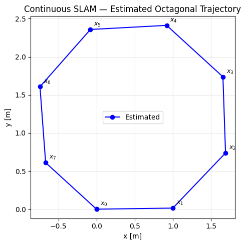

Example 3 — Hybrid Inference: Uncertain Motion Mode¶

Problem description¶

A robot moves from $x_0$ to $x_1$ to $x_2$ . The first odometry step has an uncertain mode $D_0 \in \{0, 1\}$ :

Mode 0 (normal): Reliable motion $\Delta x = (1, 0, 0)$ with small noise.
Mode 1 (slippery): Same nominal motion but with large noise.

The second odometry step is a known, pure-continuous BetweenFactorPose2.

A DecisionTreeFactor encodes a prior over the mode, and we also add a discrete observation factor that says mode 0 is very likely. After calling DCSAM.update(), we verify that:

The discrete estimate is $\hat{D}_0 = 0$ (normal mode).
The continuous estimates are close to the ground truth.

# ---- Noise models ----
tight_noise = noiseModel.Isotropic.Sigma(3, 0.1)   # normal motion
loose_noise = noiseModel.Isotropic.Sigma(3, 2.0)   # slippery surface

# ---- Ground-truth motion ----
true_odom = Pose2(1.0, 0, 0)  # 1 m forward

# ---- Hybrid factor for the first odometry step ----
# Mode 0 → tight noise,  Mode 1 → loose noise
mode_key = D(0)
dk = (mode_key, 2)

odom_normal   = BetweenFactorPose2(X(0), X(1), true_odom, tight_noise)
odom_slippery = BetweenFactorPose2(X(0), X(1), true_odom, loose_noise)
hybrid_odom   = HybridNonlinearFactor(dk, [odom_normal, odom_slippery])

# ---- Graph ----
hfg = HybridNonlinearFactorGraph()

# Prior on x0 at the origin
hfg.push_back(PriorFactorPose2(X(0), Pose2(0, 0, 0),
                                noiseModel.Isotropic.Sigma(3, 0.01)))

# Hybrid first step
hfg.push_back(hybrid_odom)

# Known second step
hfg.push_back(BetweenFactorPose2(X(1), X(2), true_odom, tight_noise))

# Discrete prior: mode 0 (normal) is much more probable
hfg.push_back(DecisionTreeFactor(dk, "0.8 0.2"))

# Discrete observation: strong evidence for mode 0
hfg.push_back(DecisionTreeFactor(dk, "0.99 0.01"))

# ---- Initial guess ----
init_values = Values()
init_values.insert(X(0), Pose2(0, 0, 0))
init_values.insert(X(1), Pose2(1, 0, 0))  # nominal guess
init_values.insert(X(2), Pose2(2, 0, 0))

init_discrete = DiscreteValues()
init_discrete[mode_key] = 0

initial_guess = HybridValues(VectorValues(), init_discrete, init_values)

# ---- Solve ----
dcsam_hybrid = DCSAM()
dcsam_hybrid.update(hfg, initial_guess)
result_hybrid = dcsam_hybrid.calculateEstimate()

# Run a second iteration to refine
dcsam_hybrid.update()
result_hybrid = dcsam_hybrid.calculateEstimate()

print("Hybrid inference result")
print(f"  Discrete mode D(0): {result_hybrid.atDiscrete(mode_key)}  (expected 0 = normal)")
for i in range(3):
    p = result_hybrid.nonlinear().atPose2(X(i))
    print(f"  X({i}): x={p.x():.4f}, y={p.y():.4f}, θ={p.theta():.4f} rad")

Hybrid inference result
  Discrete mode D(0): 0  (expected 0 = normal)
  X(0): x=0.0000, y=0.0000, θ=0.0000 rad
  X(1): x=1.0000, y=0.0000, θ=0.0000 rad
  X(2): x=2.0000, y=0.0000, θ=0.0000 rad

# Visualize hybrid SLAM result
hybrid_xs = [result_hybrid.nonlinear().atPose2(X(i)).x() for i in range(3)]
hybrid_ys = [result_hybrid.nonlinear().atPose2(X(i)).y() for i in range(3)]
gt_xs = [0.0, 1.0, 2.0]
gt_ys = [0.0, 0.0, 0.0]

fig, ax = plt.subplots(figsize=(7, 3))
ax.plot(gt_xs, gt_ys, 'k--o', markersize=8, label='Ground truth')
ax.plot(hybrid_xs, hybrid_ys, 'b-s', markersize=8, label='DCSAM estimate')
for i in range(3):
    ax.annotate(f'$x_{i}$', (hybrid_xs[i], hybrid_ys[i]),
                textcoords='offset points', xytext=(5, 8), fontsize=11)
mode_label = 'normal' if result_hybrid.atDiscrete(mode_key) == 0 else 'slippery'
ax.set_xlabel('x [m]')
ax.set_ylabel('y [m]')
ax.set_title(f'Hybrid SLAM — Estimated Mode: {mode_label} (D(0)={result_hybrid.atDiscrete(mode_key)})')
ax.legend()
ax.set_ylim(-0.5, 0.5)
ax.grid(True, alpha=0.3)
plt.tight_layout()
plt.show()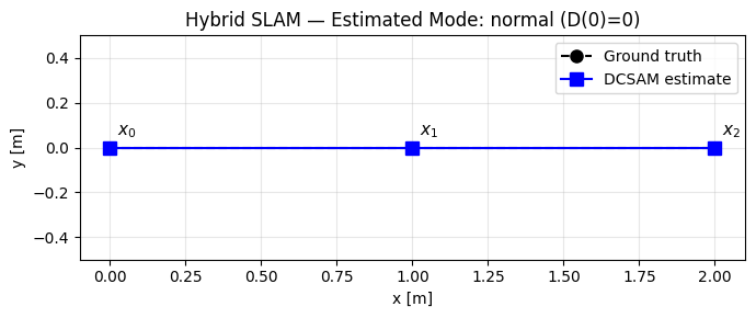

Details¶

DCSAM performed two rounds of alternating minimization:

Round 1:
- Continuous: given the initial discrete guess (mode 0), iSAM2 pulls all poses towards the odometry mean.
- Discrete: the DiscreteBoundaryFactor computed from the tight-noise component has a smaller negative log-likelihood at the current poses than the loose-noise component, so mode 0 is retained.
Round 2 (dcsam.update() with no new factors):
- Both steps refine slightly; the result converges.

The key insight is that DCSAM jointly estimates where the robot is and which motion model was active — something that neither a pure-continuous nor a pure-discrete solver can do alone.

Summary¶

Example	Variables	Method
Discrete-only	$D_1 \in \{0,1\}$	`DCSAM.update(graph, DiscreteValues)`
Continuous-only	$x_0 \ldots x_7 \in SE(2)$	`DCSAM.update(graph, HybridValues)`
Hybrid	$x_0, x_1, x_2 \in SE(2)$ , $D_0 \in \{0,1\}$	`DCSAM.update(graph, HybridValues)`

Key classes used:

HybridNonlinearFactorGraph — container for all factor types.
HybridNonlinearFactor — selects a NoiseModelFactor for each mode.
DecisionTreeFactor — probability table over discrete variables.
DCSAM — alternating-minimization solver.
HybridValues — container for the joint estimate (nonlinear(), discrete(), continuous()).