LQR Example¶

This notebook demonstrates how to solve a finite-horizon Linear Quadratic Regulator (LQR) problem using a Gaussian Factor Graph in GTSAM. The goal is to minimize a quadratic cost w.r.t. dynamics constraints over a linear dynamical system using factor-graph-based optimization. The results are compared against results from classical Riccati equations. Adapted from https://gtsam.org/2019/11/07/lqr-control.html

Author(s): Zhouyu Zhang

Authors: Frank Dellaert, et al. (see THANKS for the full author list)

See LICENSE for the license information

# In colab install gtsam and gtbook
try:
    import google.colab
    %pip install --quiet gtsam-develop
    %pip install --quiet gtbook
except ImportError:
    pass # Not in Colab

Proceed (Y/n)? y
Proceed (Y/n)? y

# Import required libraries
import numpy as np
import matplotlib.pyplot as plt
import gtsam
from gtsam import symbol
from gtsam.symbol_shorthand import X, U
import graphviz
from gtbook.display import show

Discrete-Time State-Space Form (2D State: Position and Velocity)¶

We look to work on a 1D double integrator system, in this sense, we define the state and input as:

x_k = \begin{bmatrix} x \\ \dot{x} \end{bmatrix}, \quad u_k = \ddot{x}

(1)

We can think of it as a linear vehicle for which we can control the gas paddle (acceleration). Then the discrete-time dynamics become:

x_{k+1} = A x_k + B u_k

(2)

Where:

A = \begin{bmatrix} 1 & \Delta t \\ 0 & 1 \end{bmatrix}, \quad B = \begin{bmatrix} \frac{1}{2} \Delta t^2 \\ \Delta t \end{bmatrix}

(3)

So:

\begin{bmatrix} x_{k+1} \\ \dot{x}_{k+1} \end{bmatrix} = \begin{bmatrix} 1 & \Delta t \\ 0 & 1 \end{bmatrix} \begin{bmatrix} x_k \\ \dot{x}_k \end{bmatrix} + \begin{bmatrix} \frac{1}{2} \Delta t^2 \\ \Delta t \end{bmatrix} u_k

(4)

LQR Problem Setup¶

We seek to minimize the infinite-horizon cost function:

J = \sum_{k=0}^\infty \left( x_k^\top Q x_k + u_k^\top R u_k \right)

(5)

Choose the weighting matrices:

Q = \begin{bmatrix} q_1 & 0 \\ 0 & q_2 \end{bmatrix}, \quad R = r

(6)

$Q \succeq 0$ : penalizes position and velocity
$R \succ 0$ : penalizes control effort

# Define system dynamics: x_{k+1} = A x_k + B u_k
A = np.array([[1.0, 0.1],
        [0.0, 1.0]])
B = np.array([[0.005],
        [1.0]])

# Define cost matrices: minimize sum of (xᵀQx + uᵀRu)
Q = np.eye(2)
R = np.array([[1.0]])

Graphical Model Representation of Finite-Horizon LQR¶

We formulate the finite-horizon Linear Quadratic Regulator (LQR) problem as a factor graph, allowing us to interpret optimal control as a maximum a posteriori (MAP) estimation problem.

Problem Statement¶

Given discrete-time linear dynamics:

x_{k+1} = A x_k + B u_k

(7)

and a quadratic cost function:

J(x, u) = \sum_{k=0}^{N-1} \left( x_k^\top Q x_k + u_k^\top R u_k \right) + x_N^\top Q x_N

(8)

we aim to find the state-control sequence $\{x_k, u_k\}_{k=0}^{N-1}$ minimizing $J$ , subject to initial state $x_0$ and dynamics.

MAP Estimation View¶

This control problem is equivalent to a MAP estimation over a factor graph:

\arg\max_{x_{0:N}, u_{0:N-1}} \; p(x_{0:N}, u_{0:N-1} \mid \text{costs, dynamics})

(9)

This posterior can be written as a product of factors:

p(x, u) \propto \phi_0(x_0) \prod_{k=0}^{N-1} \phi_Q(x_k) \phi_R(u_k) \phi_f(x_k, u_k, x_{k+1}) \cdot \phi_Q(x_N)

(10)

Prior Factor (Initial Condition)¶

We encode the prior on the initial state as a Gaussian:

\phi_0(x_0) \propto \exp\left( -\frac{1}{2} \| x_0 - x_{\text{init}} \|^2_{\Sigma_0} \right)

(11)

where $\Sigma_0 \approx 0 \cdot I$ enforces the initial condition tightly.

Quadratic Cost Factors¶

Each quadratic cost $x_k^\top Q x_k$ is rewritten via Cholesky decomposition $Q = L_x^\top L_x$ as:

x_k^\top Q x_k = \| L_x x_k \|^2 \quad \Rightarrow \quad \phi_Q(x_k) \propto \exp\left( -\frac{1}{2} \| L_x x_k \|^2 \right)

(12)

Similarly, for control:

\phi_R(u_k) \propto \exp\left( -\frac{1}{2} \| L_u u_k \|^2 \right), \quad R = L_u^\top L_u

(13)

These are soft constraints, penalizing deviation from zero.

Dynamics Constraints (Hard Constraints)¶

Each dynamics equation:

x_{k+1} = A x_k + B u_k

(14)

is encoded as a hard constraint, modeled as a Gaussian with zero variance:

\phi_f(x_k, u_k, x_{k+1}) \propto \delta(x_{k+1} - A x_k - B u_k) = \lim_{\Sigma \to 0} \exp\left( -\frac{1}{2} \| x_{k+1} - A x_k - B u_k \|^2_{\Sigma} \right)

(15)

This enforces the equality exactly during optimization.

Terminal Cost¶

The terminal cost is also encoded as a soft quadratic factor:

\phi_Q(x_N) \propto \exp\left( -\frac{1}{2} \| L_x x_N \|^2 \right)

(16)

# Horizon of the problem (i.e. how many discrete timesteps we want to consider)
# Note that in python the initial index starts at 0, so the terminal states would be N-1
N = 4
# Cost factors: L such that Q = LᵀL
Lx = np.linalg.cholesky(Q)
Lu = np.linalg.cholesky(R)

# Create a Gaussian factor graph for the linear-quadratic problem
graph = gtsam.GaussianFactorGraph()
initial_values = gtsam.Values()

# Set initial state: x_0 = [0, 1]^T, add a strong prior factor to fix the initial state
x0 = np.array([0.0, 1.0])
prior_noise = gtsam.noiseModel.Isotropic.Sigma(2, 1e-20)
graph.add(gtsam.JacobianFactor(X(0), np.eye(2), x0, prior_noise))

# Cost + dynamics
for k in range(N):
    xk = X(k)
    uk = U(k)

    # Cost factor: x_k^T Q x_k
    graph.add(gtsam.JacobianFactor(xk, Lx, np.zeros(2), gtsam.noiseModel.Unit.Create(2)))

    # Cost factor: u_k^T R u_k, note that there is no cost term for terminal input
    if k < N-1:
        graph.add(gtsam.JacobianFactor(uk, Lu, np.zeros(1), gtsam.noiseModel.Unit.Create(1)))

    # Dynamics hard constraint factor: x_{k+1} = A x_k + B u_k
    if k <= N-2:
        xk1 = X(k+1)
        graph.add(gtsam.JacobianFactor(
            xk1, np.eye(2),
            xk, -A,
            uk, -B,
            np.zeros((2, 1)),
            gtsam.noiseModel.Diagonal.Sigmas(np.zeros(2))  # hard constraint
        ))

# Terminal cost: x_N-1^T Q x_N-1
xN = X(N-1)
graph.add(gtsam.JacobianFactor(xN, Lx, np.zeros(2), gtsam.noiseModel.Unit.Create(2)))

# Solve the factor graph and retrieve the results
result = graph.optimize()

states = []
controls = []
for k in range(N):
    xk = X(k)
    uk = U(k)
    states.append(result.at(xk))
    if k < N-1:
      controls.append(result.at(uk))


states = np.array(states)
controls = np.array(controls)

# Plotting
plt.figure(figsize=(10, 4))
plt.plot(states[:, 0], label='Position')
plt.plot(states[:, 1], label='Velocity')
plt.title('GTSAM-solved State Trajectories')
plt.legend()
states

array([[0.        , 1.        ],
       [0.0968027 , 0.36053946],
       [0.13167395, 0.12400146],
       [0.14365837, 0.04085496]])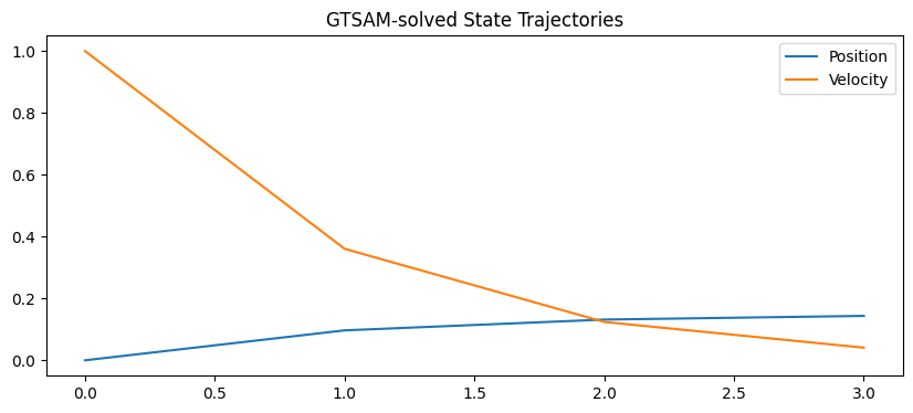

Visualizing the Factor Graph and Variable Elimination (Bayes Net)¶

Initial Factor Graph¶

The first plot generated by graphviz.Source(graph.dot()) visualizes the factor graph representation of the LQR problem.

Ellipses represent variable nodes: states $x_k$ and controls $u_k$ .
Black dots are factor nodes connecting variables — each represents either:
- A cost factor (state or control penalty),
- A dynamics constraint,
- Or a prior (for $x_0$ ).

The structure reflects the temporal nature of the problem:

Each state $x_k$ is connected to its predecessor and successor via dynamics,
Each control $u_k$ connects two consecutive states,
Cost factors attach individually to each $x_k$ and $u_k$ .

graphviz.Source(graph.dot())

Loading...

From Factor Graph to Bayes Net via Variable Elimination¶

After constructing a Gaussian factor graph to represent the finite-horizon LQR problem, we can use GTSAM’s eliminateSequential(ordering) to transform the factor graph into a Bayes Net — a directed acyclic graphical model representing the posterior distribution over all variables in a factored form.

The following plots will visualize the Bayes Net obtained using the elimination order:

\text{Ordering} = [x_0, u_0, x_1, u_1, x_2, u_2, x_3]

(17)

Structure of the Bayes Net¶

Each node in the plot represents a variable, and each arrow represents a dependency in a conditional Gaussian distribution arising from the variable elimination process. For example:

$x_2 \leftarrow \{x_3, u_2\}$
⇒ $p(x_2 \mid x_3, u_2)$
$u_1 \leftarrow \{x_2\}$
⇒ $p(u_1 \mid x_2)$

This structure means that once we solve for the “latest” variable (e.g., $x_3$ ), we can back-substitute through the DAG to recover the entire trajectory.

What Does Elimination Do?¶

In mathematical terms, elimination rewrites the joint Gaussian density:

$p(x_0, u_0, x_1, u_1, \dots, x_N) \propto \prod_i \phi_i(x_i, u_i)$

as a sequence of conditionals:

$p(x_0, u_0, x_1, \dots) = p(x_3) \cdot p(x_2 \mid x_3, u_2) \cdot \dots \cdot p(x_0)$

Each conditional is Gaussian:

$x_k = A_k \cdot \text{Parents}(x_k) + \eta_k, \quad \eta_k \sim \mathcal{N}(0, \Sigma_k)$

This allows us to represent the problem as a triangular system, suitable for efficient solving.

Effect of Elimination Ordering¶

Will the result (optimal trajectory) change if we change the elimination ordering?¶

No — the MAP solution is invariant under ordering for linear-Gaussian systems, because the solution to:

\min_x \|Ax - b\|^2

(18)

is unique and does not depend on the factorization path.

What changes?¶

Structure of the Bayes Net:
The set of conditionals and their dependencies change. E.g., if we eliminate all controls first, each $u_k$ may depend on more than just $x_k$ , introducing wider conditionals.
Computational efficiency:
Different orderings lead to different fill-in patterns during matrix factorization (e.g., Cholesky). A poor ordering increases memory and time.
Sparsity pattern:
An optimized ordering (e.g., using COLAMD or METIS) maintains sparse Jacobians and minimal cross-dependencies.
Numerical stability (nonlinear problems):
Poor ordering may lead to ill-conditioned systems or less stable Gauss-Newton updates.

Analogy to QR/Cholesky¶

The process is equivalent to structured Gaussian elimination or QR factorization of the system $Ax = b$ , where variable elimination corresponds to pivoting rows and columns of the matrix in a specific order.

ordering = gtsam.Ordering()
for k in range(N):
  ordering.push_back(X(k))
  if k < N-1:
    ordering.push_back(U(k))


# Generate a reversed ordering from above order
ordering_reversed = gtsam.Ordering()
for k in range(N-1, -1, -1):
  ordering_reversed.push_back(X(k))
  if k > 0:
    ordering_reversed.push_back(U(k-1))



print("Ordering:", ordering_reversed)

Ordering: Position 0: x3, u2, x2, u1, x1, u0, x0

dag = graph.eliminateSequential(ordering_reversed)
show(dag, hints={"u":1, "x":0})

Loading...

# The sparse matrix reprenstation of the system
plt.imshow(graph.jacobian(ordering)[0][2:,:], cmap="RdYlGn")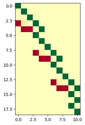

# The resulting Bayesian graph under a different ordering
# The resulting dependency would change, like we have described before

# New ordering
N = 4
ordering = gtsam.Ordering()
for k in range(N-1, -1, -1):
  ordering.push_back(X(k))
for k in range(N-1, -1, -1):
  if k > 0:
    ordering.push_back(U(k-1))
print("New Ordering:", ordering)
dag = graph.eliminateSequential(ordering)
show(dag, hints={"u":1, "x":0})

Loading...

Solving the LQR Problem via the Discrete-Time Riccati Equation¶

This code solves a finite-horizon Linear Quadratic Regulator (LQR) problem using the classical backward Riccati recursion followed by a forward rollout of optimal control inputs.

Backward Riccati Recursion¶

We compute the optimal feedback gain $K_t$ by solving the discrete Riccati equation backward from the terminal cost:

S_t = R + B^\top P_{t+1} B

(19)

K_t = S_t^{-1} B^\top P_{t+1} A

(20)

P_t = Q + A^\top P_{t+1} A - A^\top P_{t+1} B K_t

(21)

The recursion builds the list of gains $K_0, K_1, K_2$ , used to compute the optimal control law $u_t = -K_t x_t$ .

Forward Rollout of the Trajectory¶

Given the initial state $x_0$ and feedback gains:

Compute each optimal control input:
$u_t = -K_t x_t$
Apply dynamics to get the next state:
$x_{t+1} = A x_t + B u_t$

This yields the full trajectory of states and controls.

# Solve the LQR problem with the classical Riccati equation method
import numpy as np
import matplotlib.pyplot as plt
from scipy.linalg import solve_discrete_are

# System definition
A = np.array([[1.0, 0.1],
        [0.0, 1.0]])
B = np.array([[0.005],
        [1.0]])
Q = np.eye(2)
R = np.array([[1.0]])
x0 = np.array([0.0, 1.0])
N = 3  # Input horizon length (state horizon would be N+1=4)

# Backward Riccati recursion to compute K_t
P = Q.copy()  # Terminal cost
K_list = []

for _ in range(N):
    S = R + B.T @ P @ B
    K = np.linalg.solve(S, B.T @ P @ A)  # K = (R + Bᵀ P B)⁻¹ Bᵀ P A
    K_list.insert(0, K)  # prepend to use forward later
    P = Q + A.T @ P @ A - A.T @ P @ B @ K  # update P for next step

# Forward rollout of trajectory
x = x0.reshape(-1, 1)
states = [x.flatten()]
controls = []

for K in K_list:
    u = -K @ x
    controls.append(u.flatten())
    x = A @ x + B @ u
    states.append(x.flatten())

states = np.array(states)
controls = np.array(controls)

# Plot
plt.figure(figsize=(10, 4))
plt.plot(states[:, 0], label='Position')
plt.plot(states[:, 1], label='Velocity')
plt.title('Riccat-equation-solved State Trajectories')
plt.xlabel('Time step')
plt.legend()


plt.tight_layout()
plt.show()

# Optional: print values
print("States:\n", states)
print("Controls:\n", controls)

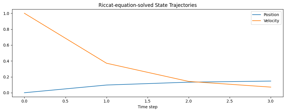
States:
 [[0.         1.        ]
 [0.09685631 0.37126203]
 [0.13283732 0.14222434]
 [0.14670236 0.07074541]]
Controls:
 [[-0.62873797]
 [-0.22903769]
 [-0.07147893]]