EqVIO Equivariant Filter Example

An Equivariant Filter for Visual-Inertial Odometry¶

This notebook demonstrates the Equivariant Filter (EqF) for state estimation in a visual-inertial odometry context, based on the paper:

“EqVIO: An Equivariant Filter for Visual Inertial Odometry” by van Goor et al.

In this tutorial, we will utilize a subset of the EuRoC MAV dataset, which is a series of stereo images and synchronized IMU measurements collected on micro-aerial-vehicles (MAVs). We will:

load a processed 60 second EqVIO replay log,
step through EqVIOFilter construction and the replay loop that calls initializeFromIMU, predict, and update,
compare the estimated translation trajectory against EuRoC ground truth in 3D, and
compare the estimated velocity against EuRoC ground truth over time.

This demo uses the gtsam_unstable.EqVIOFilter class which provides a clean interface for predict/update operations.

Note: CSV parsing, IMU segmentation helpers, and plotting utilities are tucked into a collapsible cell; the filter driver itself is written out in the main narrative cells.

Try it out in Colab!

Setup and Imports¶

We will use:

gtsam_unstable.eqvio for the filter
plotly for plotting
the processed replay CSV for IMU and feature measurements
the original EuRoC ground-truth CSV for clean pose and velocity references

The data files are located in this AwesomeEqF repository under the data folder.


from __future__ import annotations

from dataclasses import dataclass, field
from pathlib import Path
import csv
import math
from typing import Dict, List, Optional

import plotly.graph_objects as go
from plotly.subplots import make_subplots
import numpy as np

import gtsam
import gtsam_unstable

Grab the Input Files¶

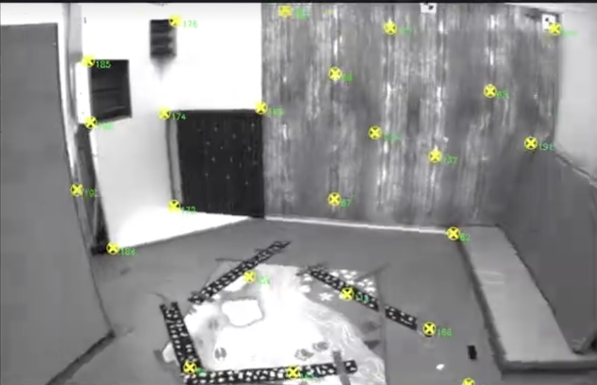
We preprocess the EuRoC MAV dataset such that the first 60 seconds of Vicon Room 1 are available to us in eqvio_processed_60s.csv. Our preprocessing runs GIFT (a library developed by van Goor to perform invariant feature tracking) as well so that we can abstract away the minutae and focus on the filter logic. Here’s what the feature tracker looks like visually, with sampled points being tracked over time as the MAV moves through the room:

We also obtain the ground truth data from the published EuRoC dataset to compare against the filter output.

def _data_dir() -> Path:
    """Resolve repo `data/` from cwd (repo root or `notebooks/`)."""
    start = Path.cwd().resolve()
    for directory in (start, *start.parents):
        data = directory / "data"
        if (data / "eqvio_processed_60s.csv").is_file():
            return data
    raise FileNotFoundError(
        f"Could not find data/eqvio_processed_60s.csv under {start} or its parents. "
        "cd to the AwesomeEqF repository root and re-run."
    )

_DATA = _data_dir()
REPLAY_CSV = _DATA / "eqvio_processed_60s.csv"
GROUNDTRUTH_CSV = _DATA / "eqvio_ground_truth.csv"

REPLAY_CSV, GROUNDTRUTH_CSV

(PosixPath('/Users/apollo/dev/research/borg/AwesomeEqF/data/eqvio_processed_60s.csv'),
 PosixPath('/Users/apollo/dev/research/borg/AwesomeEqF/data/eqvio_ground_truth.csv'))

Data Structures¶

The processed replay log makes use of three kinds of rows:

meta rows for configuration and calibration,
imu rows for inertial samples, and
vision_feature rows for tracked feature bearings.

We load those into simple Python dataclasses so the replay logic stays easy to read.


@dataclass
class ReplayEvent:
    kind: str
    seq: int
    t_abs: float
    t_rel: float = 0.0
    frame_idx: int = -1
    imu: Optional[gtsam_unstable.eqvio.IMUInput] = None
    vision: Dict[int, np.ndarray] = field(default_factory=dict)


@dataclass
class ReplayLog:
    metadata: Dict[str, str]
    events: List[ReplayEvent]


@dataclass
class GroundTruthTrajectory:
    t_abs: np.ndarray
    position_world: np.ndarray
    quaternion_wxyz: np.ndarray
    velocity_world: np.ndarray


@dataclass
class BufferedImuPropagation:
    imu_inputs: List[gtsam_unstable.eqvio.IMUInput] = field(default_factory=list)
    dts: List[float] = field(default_factory=list)
    propagated_time: float = 0.0
    trim_count: int = 0


@dataclass
class TimestampedImu:
    t_abs: float
    imu: gtsam_unstable.eqvio.IMUInput


@dataclass
class RigidAlignment:
    rotation: np.ndarray
    translation: np.ndarray


@dataclass
class ReplayResults:
    t_abs: np.ndarray
    t_rel: np.ndarray
    est_position: np.ndarray
    est_velocity: np.ndarray
    gt_position_world: np.ndarray
    gt_position_aligned: np.ndarray
    gt_velocity_body: np.ndarray
    alignment: RigidAlignment
    measurement_noise_variance: float
    final_landmark_count: int


def _parse_float(text: str, fallback: float = 0.0) -> float:
    if text is None or text == '':
        return fallback
    return float(text)


def _parse_int(text: str, fallback: int = 0) -> int:
    if text is None or text == '':
        return fallback
    return int(text)


def _metadata_finite_float(metadata: Dict[str, str], key: str, fallback: float) -> float:
    if key not in metadata or metadata[key] == '':
        return fallback
    try:
        value = float(metadata[key])
        return value if math.isfinite(value) else fallback
    except ValueError:
        return fallback


def _required_columns() -> List[str]:
    return [
        'row_type',
        't_abs',
        't_rel',
        'seq',
        'frame_idx',
        'landmark_id',
        'gx',
        'gy',
        'gz',
        'ax',
        'ay',
        'az',
        'bgx',
        'bgy',
        'bgz',
        'bax',
        'bay',
        'baz',
        'u_norm',
        'v_norm',
        'key',
        'value',
    ]


def read_replay_csv(csv_path: Path) -> ReplayLog:
    metadata: Dict[str, str] = {}
    events: List[ReplayEvent] = []
    seq_to_vision_event: Dict[int, int] = {}

    with csv_path.open(newline='', encoding='utf-8') as handle:
        reader = csv.DictReader(handle)
        if reader.fieldnames is None:
            raise ValueError(f'Empty replay CSV: {csv_path}')

        for key in _required_columns():
            if key not in reader.fieldnames:
                raise ValueError(f'Missing required replay column: {key}')

        for row in reader:
            row_type = (row.get('row_type') or '').strip()
            if not row_type:
                continue

            if row_type == 'meta':
                key = (row.get('key') or '').strip()
                if key:
                    metadata[key] = (row.get('value') or '').strip()
                continue

            seq = _parse_int(row.get('seq'), 0)
            t_abs = _parse_float(row.get('t_abs'), 0.0)
            t_rel = _parse_float(row.get('t_rel'), 0.0)

            if row_type == 'imu':
                imu = gtsam_unstable.eqvio.IMUInput()
                imu.stamp = t_abs
                imu.gyr = np.array([
                    _parse_float(row.get('gx')),
                    _parse_float(row.get('gy')),
                    _parse_float(row.get('gz')),
                ])
                imu.acc = np.array([
                    _parse_float(row.get('ax')),
                    _parse_float(row.get('ay')),
                    _parse_float(row.get('az')),
                ])
                imu.gyrBiasVel = np.array([
                    _parse_float(row.get('bgx')),
                    _parse_float(row.get('bgy')),
                    _parse_float(row.get('bgz')),
                ])
                imu.accBiasVel = np.array([
                    _parse_float(row.get('bax')),
                    _parse_float(row.get('bay')),
                    _parse_float(row.get('baz')),
                ])
                events.append(ReplayEvent(kind='imu', seq=seq, t_abs=t_abs, t_rel=t_rel, imu=imu))
                continue

            if row_type == 'vision_feature':
                frame_idx = _parse_int(row.get('frame_idx'), -1)
                landmark_id = _parse_int(row.get('landmark_id'), 0)
                u_norm = _parse_float(row.get('u_norm'), 0.0)
                v_norm = _parse_float(row.get('v_norm'), 0.0)

                if seq not in seq_to_vision_event:
                    event = ReplayEvent(
                        kind='vision',
                        seq=seq,
                        t_abs=t_abs,
                        t_rel=t_rel,
                        frame_idx=frame_idx,
                        vision={landmark_id: np.array([u_norm, v_norm])},
                    )
                    seq_to_vision_event[seq] = len(events)
                    events.append(event)
                else:
                    event = events[seq_to_vision_event[seq]]
                    event.vision[landmark_id] = np.array([u_norm, v_norm])
                continue

            raise ValueError(f'Unknown row_type: {row_type}')

    events.sort(key=lambda event: event.seq)
    return ReplayLog(metadata=metadata, events=events)


def read_groundtruth_csv(csv_path: Path) -> GroundTruthTrajectory:
    t_abs: List[float] = []
    position_world: List[np.ndarray] = []
    quaternion_wxyz: List[np.ndarray] = []
    velocity_world: List[np.ndarray] = []

    with csv_path.open(newline='', encoding='utf-8') as handle:
        reader = csv.reader(handle)
        header = next(reader, None)
        if header is None:
            raise ValueError(f'Empty ground-truth CSV: {csv_path}')

        for row in reader:
            t_abs.append(float(row[0]) * 1e-9)
            position_world.append(np.array([float(row[1]), float(row[2]), float(row[3])]))
            quaternion_wxyz.append(np.array([float(row[4]), float(row[5]), float(row[6]), float(row[7])]))
            velocity_world.append(np.array([float(row[8]), float(row[9]), float(row[10])]))

    return GroundTruthTrajectory(
        t_abs=np.asarray(t_abs),
        position_world=np.vstack(position_world),
        quaternion_wxyz=np.vstack(quaternion_wxyz),
        velocity_world=np.vstack(velocity_world),
    )

Load the Replay Log and EuRoC Ground Truth¶

The replay log is the compact event stream that drives the filter. The EuRoC ground-truth file gives us the reference position, orientation, and world-frame velocity trajectory we will use for evaluation.


log = read_replay_csv(REPLAY_CSV)
groundtruth = read_groundtruth_csv(GROUNDTRUTH_CSV)

imu_events = sum(event.kind == 'imu' for event in log.events)
vision_events = sum(event.kind == 'vision' for event in log.events)
vision_features = sum(len(event.vision) for event in log.events if event.kind == 'vision')

print(f'Replay events: {len(log.events)}')
print(f'IMU events: {imu_events}')
print(f'Vision frames: {vision_events}')
print(f'Vision features: {vision_features}')
print(f"Replay duration (metadata): {log.metadata.get('duration_sec', 'unknown')} s")
print(f'Ground-truth samples: {len(groundtruth.t_abs)}')

Replay events: 13202
IMU events: 12001
Vision frames: 1201
Vision features: 29531
Replay duration (metadata): 60 s
Ground-truth samples: 28712

Replay infrastructure¶

The next cell keeps CSV parsing, calibration readers, IMU buffering between camera times, and plotting utilities grouped so the next few cells can focus on the EqVIO predict / update calls.

Helpers worth skimming:

make_buffered_imu_propagation turns irregular IMU timestamps into (IMUInput, Δt) pairs from the last vision time to the current frame.
Ground-truth alignment (rigid_align_points, _body_frame_velocity, …): we rigidly align EuRoC positions for trajectory plots and express velocity in the body frame to match EqVIOFilter.velocity().

def _camera_offset_from_metadata(metadata: Dict[str, str]) -> Optional[gtsam.Pose3]:
    keys = ['T_ci_tx', 'T_ci_ty', 'T_ci_tz', 'T_ci_qw', 'T_ci_qx', 'T_ci_qy', 'T_ci_qz']
    if any(k not in metadata or metadata[k] == '' for k in keys):
        return None

    tx = float(metadata['T_ci_tx'])
    ty = float(metadata['T_ci_ty'])
    tz = float(metadata['T_ci_tz'])
    qw = float(metadata['T_ci_qw'])
    qx = float(metadata['T_ci_qx'])
    qy = float(metadata['T_ci_qy'])
    qz = float(metadata['T_ci_qz'])

    norm = math.sqrt(qw * qw + qx * qx + qy * qy + qz * qz)
    if norm <= 1e-12:
        return None
    qw /= norm
    qx /= norm
    qy /= norm
    qz /= norm

    return gtsam.Pose3(gtsam.Rot3.Quaternion(qw, qx, qy, qz), np.array([tx, ty, tz]))


def _initial_covariance_from_metadata(metadata: Dict[str, str]) -> np.ndarray:
    sigma0 = np.eye(21)

    def set_initial_variance_block(idx: int, key: str, fallback: float) -> None:
        sigma0[idx : idx + 3, idx : idx + 3] *= _metadata_finite_float(metadata, key, fallback)

    set_initial_variance_block(0, 'eqf.initial_var_bias_omega', 0.1)
    set_initial_variance_block(3, 'eqf.initial_var_bias_accel', 0.1)
    set_initial_variance_block(6, 'eqf.initial_var_attitude', 1e-4)
    set_initial_variance_block(9, 'eqf.initial_var_position', 1e-4)
    set_initial_variance_block(12, 'eqf.initial_var_velocity', 1e-2)
    set_initial_variance_block(15, 'eqf.initial_var_cam_attitude', 1e-5)
    set_initial_variance_block(18, 'eqf.initial_var_cam_position', 1e-4)
    return sigma0


def _params_from_metadata(metadata: Dict[str, str]) -> gtsam_unstable.eqvio.EqVIOFilterParams:
    params = gtsam_unstable.eqvio.EqVIOFilterParams()
    params.initialPointDepth = _metadata_finite_float(metadata, 'eqf.initial_point_depth', 10.0)
    params.initialPointVariance = _metadata_finite_float(metadata, 'eqf.initial_point_variance', 1.0)

    outlier_threshold_abs = _metadata_finite_float(metadata, 'eqf.outlier_threshold_abs', 1e8)
    outlier_threshold_abs = _metadata_finite_float(
        metadata, 'eqf.outlier_threshold_abs_norm', outlier_threshold_abs
    )
    params.outlierThresholdAbs = outlier_threshold_abs
    params.featureRetention = _metadata_finite_float(metadata, 'eqf.feature_retention', 0.3)
    params.biasOmegaProcessVariance = _metadata_finite_float(
        metadata, 'eqf.process_var_bias_omega', 0.001
    )
    params.biasAccelProcessVariance = _metadata_finite_float(
        metadata, 'eqf.process_var_bias_accel', 0.001
    )
    params.attitudeProcessVariance = _metadata_finite_float(
        metadata, 'eqf.process_var_attitude', 0.001
    )
    params.positionProcessVariance = _metadata_finite_float(
        metadata, 'eqf.process_var_position', 0.001
    )
    params.velocityProcessVariance = _metadata_finite_float(
        metadata, 'eqf.process_var_velocity', 0.001
    )
    params.cameraAttitudeProcessVariance = _metadata_finite_float(
        metadata, 'eqf.process_var_cam_attitude', 0.001
    )
    params.cameraPositionProcessVariance = _metadata_finite_float(
        metadata, 'eqf.process_var_cam_position', 0.001
    )
    params.pointProcessVariance = _metadata_finite_float(metadata, 'eqf.process_var_point', 0.001)

    input_noise = np.zeros((12, 12))
    input_variances = {
        0: _metadata_finite_float(metadata, 'eqf.input_var_gyr', 1e-3),
        3: _metadata_finite_float(metadata, 'eqf.input_var_acc', 1e-3),
        6: _metadata_finite_float(metadata, 'eqf.input_var_gyr_bias_walk', 1e-3),
        9: _metadata_finite_float(metadata, 'eqf.input_var_acc_bias_walk', 1e-3),
    }
    for idx, variance in input_variances.items():
        input_noise[idx : idx + 3, idx : idx + 3] = np.eye(3) * variance
    params.inputNoise = input_noise
    return params


def make_buffered_imu_propagation(
    imu_buffer: List[TimestampedImu], current_time: float, target_time: float
) -> BufferedImuPropagation:
    out = BufferedImuPropagation()
    if not imu_buffer or target_time <= current_time:
        return out

    t_ref = current_time
    for i, sample in enumerate(imu_buffer):
        t0 = max(sample.t_abs, t_ref)
        t1 = min(imu_buffer[i + 1].t_abs, target_time) if i + 1 < len(imu_buffer) else target_time
        dt = max(t1 - t0, 0.0)
        if dt <= 0.0:
            continue
        out.imu_inputs.append(sample.imu)
        out.dts.append(dt)
        out.propagated_time += dt

    first_ge_target = None
    for i, sample in enumerate(imu_buffer):
        if sample.t_abs >= target_time:
            first_ge_target = i
            break
    idx = len(imu_buffer) if first_ge_target is None else first_ge_target
    if idx != 0:
        out.trim_count = idx - 1

    return out


def _interp_columns(sample_times: np.ndarray, ref_times: np.ndarray, ref_values: np.ndarray) -> np.ndarray:
    return np.column_stack([
        np.interp(sample_times, ref_times, ref_values[:, i])
        for i in range(ref_values.shape[1])
    ])


def _body_frame_velocity(
    sample_times: np.ndarray,
    gt_times: np.ndarray,
    gt_quaternion_wxyz: np.ndarray,
    gt_velocity_world: np.ndarray,
) -> np.ndarray:
    velocity_world = _interp_columns(sample_times, gt_times, gt_velocity_world)
    indices = np.searchsorted(gt_times, sample_times)
    indices = np.clip(indices, 0, len(gt_times) - 1)

    velocity_body = []
    for velocity, idx in zip(velocity_world, indices):
        qw, qx, qy, qz = gt_quaternion_wxyz[idx]
        rotation = gtsam.Rot3.Quaternion(qw, qx, qy, qz)
        velocity_body.append(np.asarray(rotation.unrotate(velocity)).reshape(3))
    return np.vstack(velocity_body)


def rigid_align_points(source: np.ndarray, target: np.ndarray) -> RigidAlignment:
    source_mean = source.mean(axis=0)
    target_mean = target.mean(axis=0)
    source_centered = source - source_mean
    target_centered = target - target_mean

    U, _, Vt = np.linalg.svd(source_centered.T @ target_centered / len(source))
    rotation = Vt.T @ U.T
    if np.linalg.det(rotation) < 0:
        Vt[-1, :] *= -1
        rotation = Vt.T @ U.T

    translation = target_mean - rotation @ source_mean
    return RigidAlignment(rotation=rotation, translation=translation)


def apply_alignment(points: np.ndarray, alignment: RigidAlignment) -> np.ndarray:
    return (alignment.rotation @ points.T).T + alignment.translation


def summarize_results(results: ReplayResults) -> Dict[str, float]:
    position_errors = np.linalg.norm(results.est_position - results.gt_position_aligned, axis=1)
    velocity_errors = np.linalg.norm(results.est_velocity - results.gt_velocity_body, axis=1)
    return {
        'samples_compared': int(len(results.t_rel)),
        'overlap_start_sec': float(results.t_rel[0]),
        'overlap_end_sec': float(results.t_rel[-1]),
        'position_rmse_m': float(np.sqrt(np.mean(position_errors**2))),
        'final_position_error_m': float(position_errors[-1]),
        'velocity_rmse_mps': float(np.sqrt(np.mean(velocity_errors**2))),
        'final_velocity_error_mps': float(velocity_errors[-1]),
        'measurement_noise_variance': float(results.measurement_noise_variance),
        'final_landmark_count': int(results.final_landmark_count),
    }


def _trajectory_scene_ranges(points: np.ndarray) -> tuple[np.ndarray, float]:
    mins = points.min(axis=0)
    maxs = points.max(axis=0)
    centers = (mins + maxs) / 2.0
    span = float(np.max(maxs - mins))
    radius = 0.5 * span if span > 1e-9 else 1.0
    return centers, radius


def plot_trajectory_3d(results: ReplayResults) -> go.Figure:
    points = np.vstack([results.gt_position_aligned, results.est_position])
    centers, radius = _trajectory_scene_ranges(points)

    gt = results.gt_position_aligned
    est = results.est_position

    fig = go.Figure()
    fig.add_trace(
        go.Scatter3d(
            x=gt[:, 0],
            y=gt[:, 1],
            z=gt[:, 2],
            mode='lines',
            name='Ground truth (aligned)',
            line=dict(color='black', width=6),
        )
    )
    fig.add_trace(
        go.Scatter3d(
            x=est[:, 0],
            y=est[:, 1],
            z=est[:, 2],
            mode='lines',
            name='EqVIO estimate',
            line=dict(color='#1f77b4', width=6),
        )
    )
    for row, color, sym in (
        (gt[0], 'black', 'circle'),
        (est[0], '#1f77b4', 'circle'),
        (gt[-1], 'black', 'diamond'),
        (est[-1], '#1f77b4', 'diamond'),
    ):
        fig.add_trace(
            go.Scatter3d(
                x=[row[0]],
                y=[row[1]],
                z=[row[2]],
                mode='markers',
                marker=dict(size=9, color=color, symbol=sym),
                showlegend=False,
            )
        )

    fig.update_layout(
        title=dict(
            text='Ground Truth vs EqVIO Trajectory<br><sup>Translation component of pose</sup>',
        ),
        scene=dict(
            xaxis=dict(
                range=[centers[0] - radius, centers[0] + radius],
                title='x [m]',
            ),
            yaxis=dict(
                range=[centers[1] - radius, centers[1] + radius],
                title='y [m]',
            ),
            zaxis=dict(
                range=[centers[2] - radius, centers[2] + radius],
                title='z [m]',
            ),
            aspectmode='cube',
        ),
        margin=dict(l=0, r=0, t=60, b=0),
        legend=dict(yanchor='top', y=0.99, xanchor='left', x=0.02),
    )
    return fig


def plot_velocity_comparison(results: ReplayResults) -> go.Figure:
    fig = make_subplots(rows=4, cols=1, shared_xaxes=True, vertical_spacing=0.06)
    t = results.t_rel

    for i, label in enumerate(('x', 'y', 'z')):
        row = i + 1
        fig.add_trace(
            go.Scatter(
                x=t,
                y=results.gt_velocity_body[:, i],
                mode='lines',
                name='Ground truth',
                line=dict(color='black', width=2),
                legendgroup='gt',
                showlegend=(i == 0),
            ),
            row=row,
            col=1,
        )
        fig.add_trace(
            go.Scatter(
                x=t,
                y=results.est_velocity[:, i],
                mode='lines',
                name='EqVIO',
                line=dict(color='#1f77b4', width=2),
                legendgroup='eqvio',
                showlegend=(i == 0),
            ),
            row=row,
            col=1,
        )
        fig.update_yaxes(title_text=f'v_{label} [m/s]', row=row, col=1)

    gt_speed = np.linalg.norm(results.gt_velocity_body, axis=1)
    est_speed = np.linalg.norm(results.est_velocity, axis=1)
    fig.add_trace(
        go.Scatter(
            x=t,
            y=gt_speed,
            mode='lines',
            name='Ground truth',
            line=dict(color='black', width=2),
            legendgroup='gt',
            showlegend=False,
        ),
        row=4,
        col=1,
    )
    fig.add_trace(
        go.Scatter(
            x=t,
            y=est_speed,
            mode='lines',
            name='EqVIO',
            line=dict(color='#1f77b4', width=2),
            legendgroup='eqvio',
            showlegend=False,
        ),
        row=4,
        col=1,
    )
    fig.update_yaxes(title_text='|v| [m/s]', row=4, col=1)
    fig.update_xaxes(title_text='time [s]', row=4, col=1)

    fig.update_layout(
        title=dict(
            text='Velocity Comparison<br><sup>Body-frame ground truth vs EqVIO output</sup>',
            y=0.98,
        ),
        height=950,
        legend=dict(orientation='h', yanchor='bottom', y=1.02, xanchor='right', x=1),
    )
    return fig

Build `EqVIOFilter`¶

xi_ref is the fixed reference element on the homogeneous space. We optionally install the camera–IMU extrinsic (cameraOffset) from CSV metadata. initial_covariance scales a $21 \times 21$ template of initial uncertainties (biases, attitude, position, velocity, camera pose relative to IMU). EqVIOFilterParams holds process noise, feature retention, and other tuning read from metadata.

The camera object is a normalized pinhole: bearings in the CSV are already $(u,v)$ on the normalized image plane, so the calibration is identity-scale with zero skew and principal point at the origin. We need a camera to handle projection for tracked features in the data!

The replay keeps an IMU buffer plus gravity_initialized / current_time state that the main loop uses next.

camera_offset = _camera_offset_from_metadata(log.metadata)
initial_covariance = _initial_covariance_from_metadata(log.metadata)
params = _params_from_metadata(log.metadata)
measurement_noise_variance = _metadata_finite_float(
    log.metadata, "eqf.measurement_noise_variance_norm", 1e-4
)

xi_ref = gtsam_unstable.eqvio.State()
if camera_offset is not None:
    xi_ref.cameraOffset = camera_offset

filter_eqf: Optional[gtsam_unstable.eqvio.EqVIOFilter] = None
camera = gtsam.PinholeCameraCal3_S2(
    gtsam.Pose3(), gtsam.Cal3_S2(1.0, 1.0, 0.0, 0.0, 0.0)
)
imu_buffer: List[TimestampedImu] = []
gravity_initialized = False
current_time = -1.0

sampled_t_abs: List[float] = []
sampled_t_rel: List[float] = []
est_position: List[np.ndarray] = []
est_velocity: List[np.ndarray] = []

Main replay loop: `predict` then `update`¶

Events are sorted by sequence. IMU rows create the filter on first use, call initializeFromIMU once gravity can be inferred, and append samples to imu_buffer.

Vision rows then carry all bearing measurements for one exposure. In order, this is what happens:

make_buffered_imu_propagation converts buffer contents into inertial steps up to this frame time.
Each step calls filter_eqf.predict(imu_in, dt): the EqF is propagated piecewise for each IMU measurement between camera times.
We build measurement noise R (block $2 \times 2$ per landmark) and filter_eqf.update(event.vision, camera, R) to fuse every feature at this time.
Store translation and velocity for the plots below.

This matches the C++ EqVIOFilterExample pattern: integrate IMU between asynchronous images, then apply one visual update per frame.

for event in log.events:
    if event.kind == "imu":
        if filter_eqf is None:
            filter_eqf = gtsam_unstable.eqvio.EqVIOFilter(
                xi_ref, initial_covariance, gtsam.KeyVector(), params
            )
        if not gravity_initialized and event.imu is not None:
            filter_eqf.initializeFromIMU(event.imu)
            current_time = event.t_abs
            gravity_initialized = True
        if event.imu is not None:
            imu_buffer.append(TimestampedImu(t_abs=event.t_abs, imu=event.imu))
        continue

    if not gravity_initialized or filter_eqf is None:
        continue

    step = make_buffered_imu_propagation(imu_buffer, current_time, event.t_abs)
    for imu_in, dt in zip(step.imu_inputs, step.dts):
        filter_eqf.predict(imu_in, dt)
    if step.imu_inputs:
        current_time += step.propagated_time
    if step.trim_count > 0:
        imu_buffer = imu_buffer[step.trim_count :]

    R = np.eye(2 * len(event.vision)) * measurement_noise_variance
    filter_eqf.update(event.vision, camera, R)
    current_time = event.t_abs

    sampled_t_abs.append(event.t_abs)
    sampled_t_rel.append(event.t_rel)
    est_position.append(np.asarray(filter_eqf.position()).reshape(3))
    est_velocity.append(np.asarray(filter_eqf.velocity()).reshape(3))

if filter_eqf is None or not est_position:
    raise RuntimeError("EqVIO replay did not produce any sampled states.")

Package `ReplayResults` for evaluation¶

Keep only samples inside the ground-truth time span, interpolate EuRoC position/velocity, rigidly align translations (the filter’s world frame is arbitrary), rotate world velocity into the body frame for comparison with EqVIOFilter.velocity(), and wrap everything in ReplayResults for plotting.

gt = groundtruth
sampled_t_abs_np = np.asarray(sampled_t_abs)
sampled_t_rel_np = np.asarray(sampled_t_rel)
est_position_np = np.vstack(est_position)
est_velocity_np = np.vstack(est_velocity)

overlap_mask = (sampled_t_abs_np >= gt.t_abs[0]) & (sampled_t_abs_np <= gt.t_abs[-1])
sampled_t_abs_np = sampled_t_abs_np[overlap_mask]
sampled_t_rel_np = sampled_t_rel_np[overlap_mask]
est_position_np = est_position_np[overlap_mask]
est_velocity_np = est_velocity_np[overlap_mask]

gt_position_world = _interp_columns(sampled_t_abs_np, gt.t_abs, gt.position_world)
gt_velocity_body = _body_frame_velocity(
    sampled_t_abs_np, gt.t_abs, gt.quaternion_wxyz, gt.velocity_world
)

alignment = rigid_align_points(gt_position_world, est_position_np)
gt_position_aligned = apply_alignment(gt_position_world, alignment)

results = ReplayResults(
    t_abs=sampled_t_abs_np,
    t_rel=sampled_t_rel_np,
    est_position=est_position_np,
    est_velocity=est_velocity_np,
    gt_position_world=gt_position_world,
    gt_position_aligned=gt_position_aligned,
    gt_velocity_body=gt_velocity_body,
    alignment=alignment,
    measurement_noise_variance=measurement_noise_variance,
    final_landmark_count=filter_eqf.landmarkCount(),
)

summary = summarize_results(results)
summary

{'samples_compared': 1180,
 'overlap_start_sec': 1.0499999523162842,
 'overlap_end_sec': 60.0,
 'position_rmse_m': 0.06750979142277792,
 'final_position_error_m': 0.07123843159684429,
 'velocity_rmse_mps': 0.04277568828237973,
 'final_velocity_error_mps': 0.08379393501786624,
 'measurement_noise_variance': 1.775565600641238e-05,
 'final_landmark_count': 29}

The overlap starts a little after t_rel = 0 because the EuRoC ground-truth stream begins slightly later than the processed replay log. That is normal for this dataset slice.

Plot 1: 3D Pose Trajectory¶

This figure compares the translation component of the estimated pose against ground truth.

It is generated with Plotly, so feel free to zoom, pan, and orbit to take a look at how well the filter estimates the true position of the MAV!


plot_trajectory_3d(results)

Plot 2: Velocity Comparison¶

For velocity, we can compare more directly. The Python wrapper’s velocity() output matches a body-frame convention well, so we rotate the EuRoC world-frame velocity into the body frame using the ground-truth orientation and then plot the components over time.


plot_velocity_comparison(results)