
Overview
Differential GNSS (DGNSS) improves positioning accuracy by using a reference receiver at a precisely known location to correct errors affecting nearby GNSS users. The reference station receives the same satellite signals as the user and compares the measured ranges to the true ranges based on its known position. The differences represent combined errors from satellite clocks, orbits, and atmospheric delays. These corrections are transmitted to the user receiver, which applies them to its own measurements. Because both receivers experience nearly the same errors, especially when close together, many of these errors cancel out, reducing position errors from several meters to sub-meter or better accuracy.
GNSS positioning problems can be encoded as factor graphs in GTSAM; this notebook extends the groundwork from GNSS Single Point Positioning with Factor Graphs to improve receiver positioning accuracy using corrections from a nearby reference receiver.
Premise
We’ll use the ZOA1 station in Fremont, California to correct measurements for a nearby station, P222. Let’s download and load the satellite broadcast ephemerides and observations from both stations. Don’t forget to compute the satellite orbits 🛰
print("=== ZOA1 Data ===")
print("Downloading and extracting...", end="")
zoa1_data = gnss_utils.loadCORSRINEX([
    "https://noaa-cors-pds.s3.amazonaws.com/rinex/2026/018/brdc0180.26n.gz",
    "https://noaa-cors-pds.s3.amazonaws.com/rinex/2026/018/zoa1/zoa10180.26o.gz"
])
print("done!")
print(zoa1_data)
print("Computing satellite orbits...", end="")
zoa1_sat_pos = zoa1_data.computeSatelliteOrbits(zoa1_data.obs.data[0].time)
print("done!\n")

print("=== P222 Data ===")
print("Downloading and extracting...", end="")
p222_data = gnss_utils.loadCORSRINEX([
    "https://noaa-cors-pds.s3.amazonaws.com/rinex/2026/018/brdc0180.26n.gz",
    "https://noaa-cors-pds.s3.amazonaws.com/rinex/2026/018/p222/p2220180.26o.gz"
])
print("done!")
print(p222_data)
print("Computing satellite orbits...", end="")
p222_sat_pos = p222_data.computeSatelliteOrbits(p222_data.obs.data[0].time)
print("done!\n")
Bootstrap Initial Position
Start with PseudorangeFactor to prepare a simple factor graph for an initial baseline estimation for P222’s position. Similar to ZOA1, P222 has surveyed ground-truth coordinates to compare compare against our solution.
# Prepare factor graph:
cb_key = B(0)  # Receiver clock bias variable key.
pos_key = X(0) # Receiver position variable key.
nm = gtsam.noiseModel.Diagonal.Sigmas(np.array([1.0]))
graph = gtsam.NonlinearFactorGraph()

# Add a PseudorangeFactor for each observation:
rows = []
for obsd, sat_bias, sat_pos, pseudorange in gnss_utils.iterateObservations(p222_data, p222_sat_pos, n=7):
    graph.add(
        gtsam.PseudorangeFactor(pos_key, cb_key, pseudorange, sat_pos, sat_bias, nm)
    )

    rows.append([obsd.sat, pseudorange, obsd.time.time, 1e-3*sat_pos, sat_bias])

headers = ["Satellite", "Pseudorange (m)", "Time (unixtime seconds)", "Sat ECEF Position (km)", "Sat Clock Bias (sec)"]
print(tabulate(rows, headers=headers, tablefmt="github"))
We initialize receiver position at origin, and then use a LM solver to optimize the system.
# Solve the system:
initial_values = gtsam.Values()
initial_values.insert(cb_key, 0.0)
initial_values.insert(pos_key, np.zeros(3))
result = gtsam.LevenbergMarquardtOptimizer(graph, initial_values).optimize()

# Process the results:
clock_bias = result.atDouble(cb_key)
receiver_position = result.atVector(pos_key)
print(f"Final clock bias {clock_bias} seconds and receiver position {receiver_position} (ECEF meters)")
lon, lat, alt = ecef2lla.transform(receiver_position[0], receiver_position[1], receiver_position[2])
print(f"Latitude: {lat} degrees")
print(f"Longitude: {lon} degrees")
print(f"Altitude: {alt} meters")
gnss_utils.plotMap(lat, lon)
So far this solution passes the eye-ball test: It’s in the right US state, in roughly the correct part of the SF Bay Area. But we can quantify error by comparing the actual position of P222:
| ITRF2020 POSITION (EPOCH 2020.0)                                            |
| Computed in Apr 2025 using data through gpswk 2237.                         |
|     X =  -2689640.518 m     latitude    =  37 32 21.26653 N                 |
|     Y =  -4290437.125 m     longitude   = 122 04 59.76571 W                 |
|     Z =   3865051.027 m     ellipsoid height =   53.512   m                 |
ground_truth = np.array([-2689640.518, -4290437.125, 3865051.027]) # P222's surveyed ground-truth position.
error = ground_truth - receiver_position
print(f"Total positioning error: {np.linalg.norm(error)} meters")30 meters is a decent starting point from single-point positioning, but let’s see if we can do better.
Differential Positioning
In this scenario, we know ZOA1’s precise position ahead-of-time. Its surveyed position is published in the data portal, and reproduced here:
| ITRF2020 POSITION (EPOCH 2020.0)                                            |
| Computed in Apr 2025 using data through gpswk 2237.                         |
|     X =  -2684436.824 m     latitude    =  37 32 34.99617 N                 |
|     Y =  -4293336.957 m     longitude   = 122 00 57.42005 W                 |
|     Z =   3865351.638 m     ellipsoid height =   -3.960   m                 |
In a factor graph framework, these survey coordinates correspond to a stiff PriorFactor constraint on ZOA1’s position node to keep it anchored in the global Earth frame. The rest of the factor graph is constructed as follows:
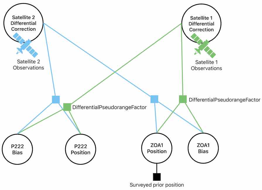
A DifferentialPseudorangeFactor is added for each receiver observation, and their correction nodes are indexed by satellite ID. For example, ZOA1’s pseudorange factor of satellite 25 links to the same correction node for P222’s pseudorange observation of satellite 25. Since different satellites are in different positions in the sky, each satellite has their own correction node to account for spatial variation in atmospheric effects. Furthermore, for long-time-series observations, the correction nodes must also account for temporal variation in the atmosphere. In that case, a linear chain of correction nodes linked with between-factors is recommended. The above structure is encoded into GTSAM below:
p222_bias_key = B(0)  # Receiver clock bias variable key.
p222_pos_key = X(0) # Receiver position variable key.
zoa1_bias_key = B(1)
zoa1_pos_key = X(1)
zoa1_ref_pos = np.array([-2684436.824, -4293336.957, 3865351.638])  # ZOA1's surveyed reference position.
nm = gtsam.noiseModel.Diagonal.Sigmas(np.array([1.0]))
graph = gtsam.NonlinearFactorGraph()

initial_values = gtsam.Values()
initial_values.insert(zoa1_pos_key, zoa1_ref_pos)
initial_values.insert(zoa1_bias_key, 0.0)
initial_values.insert(p222_pos_key, receiver_position)
initial_values.insert(p222_bias_key, clock_bias)

# Apply a prior factor constraint on zoa1's reference position:
graph.add(
    gtsam.PriorFactorVector(
        zoa1_pos_key,
        zoa1_ref_pos,
        gtsam.noiseModel.Diagonal.Sigmas(np.array([0.0005, 0.0005, 0.0005]))
    )
)

# Add factors for reference station:
sat_keymap = {}
for i, (obsd, sat_bias, sat_pos, pseudorange) in enumerate(gnss_utils.iterateObservations(zoa1_data, zoa1_sat_pos, n=40)):
    # Apply factor:
    if obsd.sat not in sat_keymap:
        initial_values.insert(C(i), 0.0)
        sat_keymap[obsd.sat] = C(i)
        correction_key = C(i)
    else:
        correction_key = sat_keymap[obsd.sat]
    factor = gtsam.DifferentialPseudorangeFactor(
            zoa1_pos_key, zoa1_bias_key, correction_key,
            pseudorange, sat_pos, sat_bias, nm)
    graph.add(factor)

# Add factors for user station:
for obsd, sat_bias, sat_pos, pseudorange in gnss_utils.iterateObservations(p222_data, p222_sat_pos, n=40):
    # Apply factor:
    if obsd.sat in sat_keymap:
        correction_key = sat_keymap[obsd.sat]
        factor = gtsam.DifferentialPseudorangeFactor(
                p222_pos_key, p222_bias_key, correction_key,
                pseudorange, sat_pos, sat_bias, nm)
        graph.add(factor)

# Solve the system:
lm = gtsam.LevenbergMarquardtOptimizer(graph, initial_values)
print(f"Initial error: {lm.error()}")
result = lm.optimize()
print(f"Final error: {lm.error()}")

# Process the results:
clock_bias = result.atDouble(p222_bias_key)
corrected_receiver_position = result.atVector(p222_pos_key)
print(f"Corrected P222 position: {corrected_receiver_position} ECEF meters")
Let’s plot these coordinates on a map, including the reference stations and single-point positions, to get a big-picture overview of how the positioning results stack up:
# Convenience plot:
lon, lat, alt = ecef2lla.transform(corrected_receiver_position[0], corrected_receiver_position[1], corrected_receiver_position[2])
print(f"Corrected geodetic coordinates: {lat}, {lon}, {alt} m")

# Center the map on P222
m = folium.Map(
    location=[lat, lon],
    zoom_start=17
)

# Plot surveyed P222 position:
folium.Circle(
    location=[37.5392407028, -122.0832682528],
    radius=10,
    tooltip="P222 Truth",
    popup="Actual P222 position"
).add_to(m)

# Plot the corrected receiver position:
folium.Marker(
    location=[lat, lon],
    tooltip="P222 Corrected",
    popup="Estimated P222 position using corrections from ZOA1",
    icon=folium.Icon(color="green", icon="plus")
).add_to(m)

# Plot the single-point-positioning solution:
lon, lat, alt = ecef2lla.transform(receiver_position[0], receiver_position[1], receiver_position[2])
folium.Marker(
    location=[lat, lon],
    tooltip="P222 SPP",
    popup="Estimated P222 position without differential corrections",
    icon=folium.Icon(color="orange", icon="minus")
).add_to(m)

# Plot ZOA1's position:
folium.Marker(
    location=[37.5430544917, -122.0159500139],
    tooltip="ZOA1",
    popup="ZOA1 reference station surveyed position",
    icon=folium.Icon(color="blue")
).add_to(m)

m
Scroll and zoom the map to get an idea for the relative positioning error between the single-point and differential solutions. The blue circle indicates the ground-truth surveyed postion of P222. The green “plus” marker shows the differentially-corrected solution. The orange “minus” marker indicates the uncorrected position. Zoom out further on the map to make the blue ZOA1 receiver position visible.
Let’s see if it’s closer to ground truth?
print(f"ZOA1 position adjustment: {1e3*np.linalg.norm(result.atVector(zoa1_pos_key) - zoa1_ref_pos)} millimeters")
error = ground_truth - corrected_receiver_position
print(f"Total positioning error: {np.linalg.norm(error)} meters")
Conclusion
98% reduction in error going from ~30 to ~0.4 meters of accuracy! The differential corrections appear to eliminate a large portion of positioning error. But we can do better! Carrier-phase data offer higher-precision measuring power, but the devil’s bargain demands an answer to the integer ambiguity problem.