Custom Factor Trajectory Localization

This notebook shows how to use gtsam.CustomFactor inside a small Pose2 trajectory problem.

Each custom factor:

touches one pose in the trajectory
stores that pose’s landmark measurements
stacks all landmark residuals into one vector
fills the analytical Jacobian using Pose2.transformTo

We then combine those custom factors with standard odometry BetweenFactorPose2 factors so the graph is a connected trajectory.

import matplotlib.pyplot as plt
import numpy as np

import gtsam
from gtsam.symbol_shorthand import X

np.set_printoptions(precision=3, suppress=True)

1. Landmarks and Noise Models¶

We use the same known landmarks for every pose. To make the plot more interesting, the landmark measurements are fairly noisy, while odometry stays reasonably accurate.

LANDMARKS = [
    np.array([5.0, 0.0]),
    np.array([2.0, 3.0]),
    np.array([6.0, 4.0]),
    np.array([8.0, 1.0]),
]

LANDMARK_SIGMA = 0.25
ODOMETRY_SIGMA_XY = 0.15
ODOMETRY_SIGMA_THETA = 0.08

LANDMARK_NOISE_MODEL = gtsam.noiseModel.Isotropic.Sigma(2 * len(LANDMARKS), LANDMARK_SIGMA)
ODOMETRY_NOISE_MODEL = gtsam.noiseModel.Diagonal.Sigmas(
    np.array([ODOMETRY_SIGMA_XY, ODOMETRY_SIGMA_XY, ODOMETRY_SIGMA_THETA])
)

print("Landmarks:")
for i, landmark in enumerate(LANDMARKS):
    print(f"  L{i}: {landmark}")

Landmarks:
  L0: [5. 0.]
  L1: [2. 3.]
  L2: [6. 4.]
  L3: [8. 1.]

2. Custom Residual Object¶

The residual object is itself the callback passed into CustomFactor. This keeps the example compact while still using analytical Jacobians.

The important trick in Python is to allocate Jacobian arrays in Fortran order before passing them into Pose2.transformTo.

class LandmarkLocalizationResidual:
    """Stack landmark errors for a single Pose2 variable."""

    def __init__(self, measurements: list[np.ndarray]):
        self.measurements = measurements

    def __call__(
        self,
        this: gtsam.CustomFactor,
        values: gtsam.Values,
        jacobians: list[np.ndarray] | None,
    ) -> np.ndarray:
        pose = values.atPose2(this.keys()[0])
        residual = np.zeros(2 * len(self.measurements))

        if jacobians is not None:
            jacobians[0] = np.zeros((2 * len(self.measurements), 3), order="F")

        for i, (landmark, measurement) in enumerate(zip(LANDMARKS, self.measurements)):
            if jacobians is not None:
                H_pose = np.zeros((2, 3), order="F")
                H_point = np.zeros((2, 2), order="F")
                predicted = pose.transformTo(landmark, H_pose, H_point)
                jacobians[0][2 * i : 2 * i + 2, :] = H_pose
            else:
                predicted = pose.transformTo(landmark)

            residual[2 * i : 2 * i + 2] = predicted - measurement

        return residual

3. Create a Noisy Trajectory Problem¶

rng = np.random.default_rng(7)


def measure_landmarks(pose: gtsam.Pose2) -> list[np.ndarray]:
    return [pose.transformTo(landmark) + rng.normal(0.0, LANDMARK_SIGMA, size=2) for landmark in LANDMARKS]


true_poses = [
    gtsam.Pose2(1.0, 2.0, 0.3),
    gtsam.Pose2(2.5, 1.0, -0.2),
    gtsam.Pose2(3.0, 2.8, 0.4),
    gtsam.Pose2(4.4, 1.6, -0.1),
]

keys = [X(i) for i in range(len(true_poses))]
measurements = [measure_landmarks(pose) for pose in true_poses]
odometry_measurements = [
    true_poses[i].between(true_poses[i + 1]).retract(
        rng.normal(0.0, [ODOMETRY_SIGMA_XY, ODOMETRY_SIGMA_XY, ODOMETRY_SIGMA_THETA])
    )
    for i in range(len(true_poses) - 1)
]

print("Landmark measurements at pose 0:")
for measurement in measurements[0]:
    print(" ", measurement)

Landmark measurements at pose 0:
  [ 3.23061308 -3.01806742]
  [1.18232223 0.43716832]
  [5.25405516 0.18516031]
  [ 6.40687112 -2.68892412]

4. Inspect One Custom Factor¶

At the ground truth, the residual is not zero anymore because we injected noise into the landmark measurements. Still, we can linearize the factor and inspect the Jacobian generated by the callback.

factor = gtsam.CustomFactor(LANDMARK_NOISE_MODEL, [keys[0]], LandmarkLocalizationResidual(measurements[0]))

values = gtsam.Values()
values.insert(keys[0], true_poses[0])

linear = factor.linearize(values)
A, b = linear.jacobian()

print("Nonlinear error:", factor.error(values))
print("Jacobian shape:", A.shape)
A

Nonlinear error: 1.9737191833686931
Jacobian shape: (8, 3)

array([[ -4.        ,   0.        , -12.37101522],
       [  0.        ,  -4.        , -12.92122217],
       [ -4.        ,   0.        ,   2.63926513],
       [  0.        ,  -4.        ,  -5.00342678],
       [ -4.        ,   0.        ,   1.73228778],
       [  0.        ,  -4.        , -21.47089144],
       [ -4.        ,   0.        , -12.09591174],
       [  0.        ,  -4.        , -25.56734087]])

5. Solve the Trajectory¶

Each pose gets one landmark CustomFactor, and consecutive poses are connected with odometry BetweenFactorPose2 factors.

graph = gtsam.NonlinearFactorGraph()

for key, measurement_set in zip(keys, measurements):
    graph.add(gtsam.CustomFactor(LANDMARK_NOISE_MODEL, [key], LandmarkLocalizationResidual(measurement_set)))

for key1, key2, odometry in zip(keys[:-1], keys[1:], odometry_measurements):
    graph.add(gtsam.BetweenFactorPose2(key1, key2, odometry, ODOMETRY_NOISE_MODEL))

initial = gtsam.Values()
for key, pose in zip(keys, true_poses):
    initial.insert(key, pose.retract(np.array([0.8, -0.6, 0.25])))

result = gtsam.LevenbergMarquardtOptimizer(graph, initial).optimize()

for i, (key, true_pose) in enumerate(zip(keys, true_poses)):
    print(f"True pose {i}:      {true_pose}")
    print(f"Estimated pose {i}: {result.atPose2(key)}")
    print()

True pose 0:      (1, 2, 0.3)

Estimated pose 0: (1.14111, 2.30025, 0.237817)


True pose 1:      (2.5, 1, -0.2)

Estimated pose 1: (2.53991, 1.15384, -0.231066)


True pose 2:      (3, 2.8, 0.4)

Estimated pose 2: (3.21574, 2.96852, 0.396358)


True pose 3:      (4.4, 1.6, -0.1)

Estimated pose 3: (4.59661, 1.6944, -0.112688)

6. Plot Ground Truth and Optimized Trajectories¶

The landmark measurements are noisy enough that the optimized trajectory does not sit exactly on top of ground truth, which makes the comparison easier to see.

def draw_pose(ax, pose: gtsam.Pose2, color: str) -> None:
    x, y, theta = pose.x(), pose.y(), pose.theta()
    ax.quiver(
        [x],
        [y],
        [np.cos(theta)],
        [np.sin(theta)],
        angles="xy",
        scale_units="xy",
        scale=1.8,
        color=color,
    )


fig, ax = plt.subplots(figsize=(7, 6))
landmarks_array = np.array(LANDMARKS)
true_xy = np.array([[pose.x(), pose.y()] for pose in true_poses])
result_xy = np.array([[result.atPose2(key).x(), result.atPose2(key).y()] for key in keys])

ax.scatter(
    landmarks_array[:, 0],
    landmarks_array[:, 1],
    marker="*",
    s=220,
    color="tab:orange",
    label="landmarks",
)

ax.plot(true_xy[:, 0], true_xy[:, 1], "-o", color="tab:green", linewidth=2, label="ground truth")
ax.plot(result_xy[:, 0], result_xy[:, 1], "-o", color="tab:blue", linewidth=2, label="optimized")

for pose in true_poses:
    draw_pose(ax, pose, "tab:green")

for key in keys:
    draw_pose(ax, result.atPose2(key), "tab:blue")

ax.set_aspect("equal", adjustable="box")
ax.set_xlabel("x (m)")
ax.set_ylabel("y (m)")
ax.set_title("Connected trajectory with CustomFactor landmark localization")
ax.grid(alpha=0.3)
ax.legend(loc="upper left")
plt.show()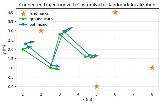

Takeaways¶

CustomFactor works well when you already know the residual you want to write.
A small callable object is often the cleanest way to package measurements and constants.
In Python, Pose2.transformTo can now provide analytical Jacobians directly when you pass Fortran-order output arrays.
Custom factors combine naturally with standard GTSAM factors such as BetweenFactorPose2 in the same trajectory graph.