GTSAM’s sfm module spans the full reconstruction pipeline: feature tracks, global rotation and translation recovery, trajectory alignment, and high-performance CPU and CUDA bundle adjustment.
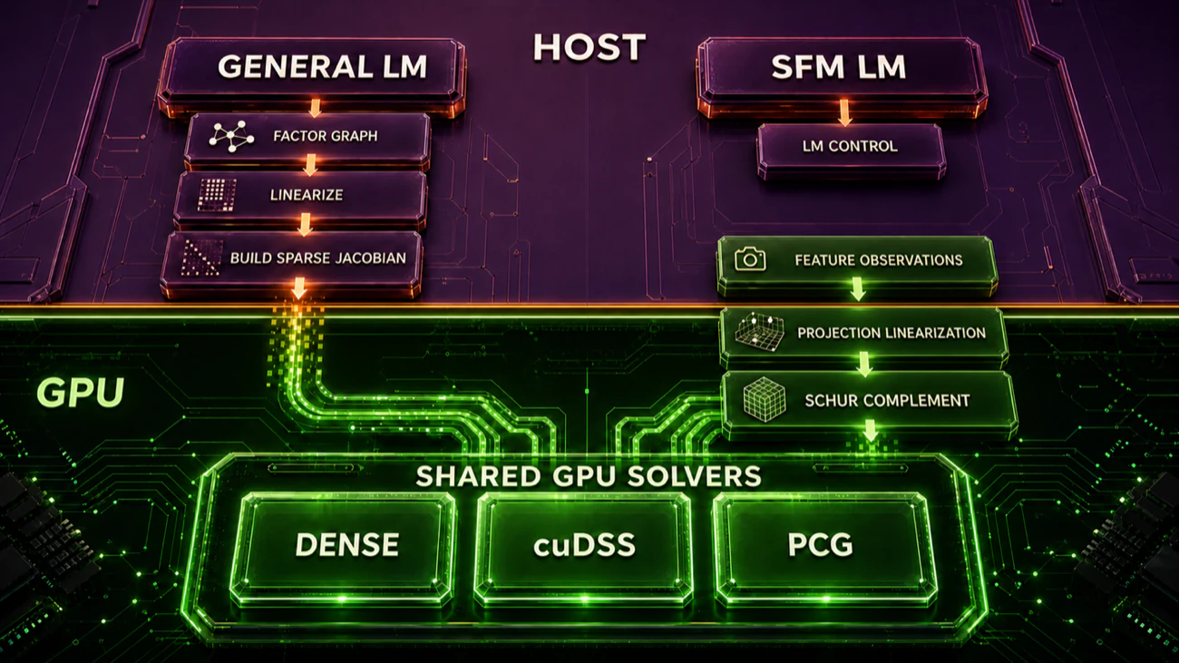
Figure 1:The general and SFM Levenberg–Marquardt paths on the GPU. The SFM optimizer uses bespoke CUDA kernels to form its camera Schur complement before dispatching to dense Cholesky, cuDSS, or PCG.
Full or Schur · standard nonlinear solver selection
Use multifrontal or sequential Cholesky/QR, MULTIFRONTAL_SOLVER, iterative PCG/SubgraphSolver, or optional CHOLMOD.
Fastest measured family: point-first MULTIFRONTAL_SOLVER (Full or Schur)
Schur today · Full mode reserved
The bespoke CUDA Schur path supports dense Cholesky, cuDSS, and PCG. Full is already part of the public API but throws a clear not-implemented exception.
Two independent choices
SfmLevenbergMarquardtOptimizer separates the elimination strategy from the linear solver:
SfmEliminationMode::Fullsolves the joint system.SfmEliminationMode::Schureliminates every activePoint3andUnit3first, then solves for all remaining variables.
CPU Schur partitioning eliminates active Point3 and Unit3 values while retaining every other value type, including poses, camera objects, and shared or per-camera calibrations. This value-based partition supports variable and global calibration without specializing the optimizer for one camera template.
CPU and CUDA defaults reflect their current fast paths and graph support. CPU defaults to Full, MULTIFRONTAL_SOLVER, and an automatically generated natural-landmark prefix followed by a METIS ordering of the reduced system; that combination was effectively tied on BAL-16, won BAL-88, and was within 0.8% of Schur on BAL-135. CUDA defaults to Schur and keeps its existing camera/Point3 backend assumptions.
| Platform | Full | Schur | Linear solvers |
|---|---|---|---|
| CPU | Supported (default) | Supported | MULTIFRONTAL_SOLVER (default), multifrontal/sequential Cholesky or QR, Iterative, optional CHOLMOD |
| CUDA | Planned; currently throws | Supported (default) | dense Cholesky, cuDSS, PCG |
CPU quick start
#include <gtsam/sfm/SfmLevenbergMarquardt.h>

gtsam::SfmLevenbergMarquardtParams params =
    gtsam::SfmLevenbergMarquardtParams::ceresDefaults();

// For the fastest measured path, graph uses point-batched projection factors.
const gtsam::Ordering reducedOrdering =
    gtsam::SfmLevenbergMarquardtOptimizer::CreateReducedOrdering(
        graph, initial);
params.setOrdering(
    gtsam::SfmLevenbergMarquardtOptimizer::CreateSchurOrdering(
        graph, reducedOrdering));

gtsam::SfmLevenbergMarquardtOptimizer optimizer(graph, initial, params);
const gtsam::Values& result = optimizer.optimize();
The Python Full-and-Schur tutorial demonstrates both elimination modes with a calibration shared by every camera. When constructing Values from NumPy arrays, use Values.insertPoint3() for landmarks so Python preserves their fixed-size Point3 type.
What Schur means for each solver
Schur mode constructs a complete ordering with a natural Point3/Unit3 prefix followed by the reduced-system ordering. One cached MultifrontalSolver factorization eliminates those landmarks, factors the Schur complement over the remaining variables, and back-substitutes through the same Bayes tree.
No reduced factor graph is created. This is mathematically the same landmark-first elimination used in Full mode when it receives the identical complete ordering; explicit Schur mode lets SFM construct that ordering from a reduced-system input.
Schur mode creates an explicit solver boundary:
MultifrontalSolver::eliminatePartialInPlace()eliminates landmarks.remainingFactorGraph()exports the reduced Hessian graph.The selected ordinary solver computes the reduced-system step.
updateSolution(reducedDelta)back-substitutes the eliminated step.
The partial-elimination symbolic state is reused across LM attempts and iterations. This path lets CHOLMOD, legacy Cholesky or QR, and iterative solvers operate on the reduced graph, at the cost of materializing reduced factors and running a separate solve.
Reduced-system ordering
In Full mode, a supplied ordering has ordinary all-variable semantics. In CPU Schur mode, supply every active key whose value is neither Point3 nor Unit3:
gtsam::Ordering reduced{pose0Key, pose1Key, globalCalibrationKey};
params.setOrdering(reduced);
Two public ordering helpers build and validate the reusable point-first ordering. CreateReducedOrdering(graph, initial) symbolically eliminates active Point3 and Unit3 values in natural key order and runs METIS on the resulting reduced graph. CreateSchurOrdering(graph, reduced) prefixes that reduced ordering with the eliminated keys; its result is the complete Schur ordering used by Full mode or the fused multifrontal path. Duplicate, missing, eliminated, and unknown reduced keys are rejected. Direct reduced solvers and iterative solvers that consume an ordering receive the same reduced-only suffix.
Select NonlinearOptimizerParams::Iterative and supply the same parameter object as an ordinary nonlinear optimizer:
PCGSolverParametersselects PCG.SubgraphSolverParametersselectsSubgraphSolverand receives the reduced-system ordering in Schur mode.Missing or unrecognized parameters throw the ordinary
NonlinearOptimizer::solveerror.
SubgraphSolver additionally requires a Gaussian graph with enough unary and binary factors to construct its spanning-tree preconditioner. Higher-arity point batches and camera clique factors do not satisfy that requirement.
The typed getLinearSolver() and setLinearSolver() conveniences coexist with the compatible string APIs.
When SuiteSparse CHOLMOD is found, NonlinearOptimizerParams::CHOLMOD works for ordinary nonlinear optimizers and both CPU SFM modes. The reusable session accepts arbitrary variable dimensions, loads ordinary Jacobian, compact batch Jacobian, and Hessian factors directly into the sparse normal system, expands key orderings into scalar permutations, and reuses symbolic analysis. Compact batches contribute their fixed-size normal blocks without a dense intermediate.
A build without CHOLMOD remains valid; selecting it produces an actionable runtime error. Constrained, non-SPD, and factorization failures are reported rather than silently falling back.
CUDA semantics
CUDA SFM currently supports only its bespoke Schur path; selecting SfmEliminationMode::Full fails immediately because full-system CUDA solving is intentionally deferred. The Schur path uses the landmark-elimination kernels shown in Figure 1, then solves the camera system with dense Cholesky, cuDSS, or PCG. CUDA orderings remain camera-only and are accepted only by backends that consume them.
Performance at a glance
The primary Release-mode benchmark compares the public CPU and CUDA fast paths on Ubuntu 24.04 with an Intel Core i7-14700F (20 physical cores, 28 logical CPUs) and 31 GiB RAM, plus an NVIDIA GeForce RTX 5060 Ti with 16 GiB VRAM. CPU values are median end-to-end optimization times from three BAL-16/BAL-88 repetitions and seven separately invoked BAL-135 runs; CUDA values are medians from three runs.
| Public optimizer path | BAL-16 s | BAL-88 s | BAL-135 s |
|---|---|---|---|
CPU Full + MULTIFRONTAL_SOLVER | 0.228 | 0.869 | 1.437 |
CPU Schur + MULTIFRONTAL_SOLVER | 0.228 | 0.873 | 1.427 |
| CUDA Schur + dense Cholesky | 0.055 | 0.218 | 0.290 |
An independent run on a Ryzen 9 5900X (12C/24T) and RTX 5090 produced the following median times; parentheses show speedup relative to CUDA schur-dense.
| Configuration | BAL-16 | BAL-88 | BAL-135 |
|---|---|---|---|
CUDA schur-dense | 0.070 | 0.200 | 0.267 |
| Schur/MultifrontalSolver | 0.412 (5.9×) | 1.505 (7.5×) | 2.115 (7.9×) |
| Full/MultifrontalSolver | 0.437 (6.2×) | 1.511 (7.6×) | 2.107 (7.9×) |
| Schur/MultifrontalCholesky | 0.643 (9.2×) | 2.232 (11.2×) | 3.012 (11.3×) |
| Schur/PCG | 0.678 (9.7×) | 2.349 (11.7×) | 3.029 (11.3×) |
Absolute times—and even the narrow Full-versus-Schur winner—vary with hardware and build, so benchmark your workload.
The timing benchmark README contains the complete solver matrices, build record, commands, timeout/unsupported results, and numerical checks.
User guides by class
Template classes appear in Python under concrete names. Wrapper-only containers adapt C++ containers at language boundaries; Python users should normally pass native lists and dictionaries as shown in the related guides.