This is the canonical structure-from-motion (SFM) example in GTSAM, and it pulls together ideas used elsewhere in this notebook series: projection factors (VisualISAMExample), the DoglegOptimizer (DogLegOptimizerExample, SelfCalibrationExample), and marginal-covariance visualization (OdometryExample) -- now applied all at once to a full 3D bundle-adjustment problem.
Unlike VisualISAMExample, which fed observations to an incremental solver one pose at a time, this notebook builds the entire factor graph up front and solves it in a single batch optimization with DoglegOptimizer. The scene is the same 10-meter landmark cube with 8 cameras circling it, this time with a known, fixed calibration.

GTSAM Copyright 2010-2026, Georgia Tech Research Corporation, Atlanta, Georgia 30332-0415 All Rights Reserved
Authors: Frank Dellaert, et al. (see THANKS for the full author list)
See LICENSE for the license information
try:
    import google.colab
    %pip install --quiet gtsam-develop
except ImportError:
    pass
import matplotlib.pyplot as plt
import numpy as np
import gtsam
from gtsam import symbol_shorthand
L = symbol_shorthand.L
X = symbol_shorthand.X
from gtsam.examples import SFMdata
from gtsam.utils import plot
from gtsam import (Cal3_S2, DoglegOptimizer, GenericProjectionFactorCal3_S2,
Marginals, NonlinearFactorGraph, PinholeCameraCal3_S2,
PriorFactorPoint3, PriorFactorPose3, Values)1. Scene and camera setup
Ground-truth landmarks and poses come from the shared SFMdata helper module, same as VisualISAMExample. Here calibration K is known and fixed -- there’s no self-calibration in this notebook.
# Define the camera calibration parameters
K = Cal3_S2(50.0, 50.0, 0.0, 50.0, 50.0)

# Define the camera observation noise model
measurement_noise = gtsam.noiseModel.Isotropic.Sigma(2, 1.0)  # one pixel in u and v

# Create the set of ground-truth landmarks
points = SFMdata.createPoints()

# Create the set of ground-truth poses
poses = SFMdata.createPoses()
2. Build the factor graph
A prior on pose x0 indirectly fixes the origin of the whole reconstruction. Then, for every pose/landmark pair, we project the ground-truth landmark through the camera to get a simulated pixel measurement, and add a GenericProjectionFactorCal3_S2 -- the same factor type used in VisualISAMExample, but here every observation goes into one graph, built entirely before optimization starts.
# Create a factor graph
graph = NonlinearFactorGraph()

# Add a prior on pose x1. This indirectly specifies where the origin is.
# 0.3 rad std on roll,pitch,yaw and 0.1m on x,y,z
pose_noise = gtsam.noiseModel.Diagonal.Sigmas(np.array([0.3, 0.3, 0.3, 0.1, 0.1, 0.1]))
factor = PriorFactorPose3(X(0), poses[0], pose_noise)
graph.push_back(factor)

# Simulated measurements from each camera pose, adding them to the factor graph
for i, pose in enumerate(poses):
    camera = PinholeCameraCal3_S2(pose, K)
    for j, point in enumerate(points):
        measurement = camera.project(point)
        factor = GenericProjectionFactorCal3_S2(measurement, measurement_noise, X(i), L(j), K)
        graph.push_back(factor)
3. Fix the scale ambiguity
SFM alone can’t distinguish a small scene photographed up close from a large scene photographed from far away -- the pixel measurements look identical either way. This is the same kind of ambiguity that makes self-calibration hard in SelfCalibrationExample, but here it’s about scale rather than focal length. A single prior on landmark l0 pins the distance between the first camera and the first landmark, and every other landmark position is interpreted relative to that scale.
point_noise = gtsam.noiseModel.Isotropic.Sigma(3, 0.1)
factor = PriorFactorPoint3(L(0), points[0], point_noise)
graph.push_back(factor)
print(graph)
NonlinearFactorGraph: size: 66
Factor 0: PriorFactor on x0
prior mean: R: [
6.12323e-17, -6.12323e-17, -1;
1, 3.7494e-33, 6.12323e-17;
-0, -1, 6.12323e-17
]
t: 30 0 0
noise model: diagonal sigmas [0.3; 0.3; 0.3; 0.1; 0.1; 0.1];
Factor 1: GenericProjectionFactor, z = [
75;
25
]
keys = { x0 l0 }
noise model: unit (2)
Factor 2: GenericProjectionFactor, z = [
62.5;
37.5
]
keys = { x0 l1 }
noise model: unit (2)
Factor 3: GenericProjectionFactor, z = [
37.5;
37.5
]
keys = { x0 l2 }
noise model: unit (2)
Factor 4: GenericProjectionFactor, z = [
25;
25
]
keys = { x0 l3 }
noise model: unit (2)
Factor 5: GenericProjectionFactor, z = [
75;
75
]
keys = { x0 l4 }
noise model: unit (2)
Factor 6: GenericProjectionFactor, z = [
62.5;
62.5
]
keys = { x0 l5 }
noise model: unit (2)
Factor 7: GenericProjectionFactor, z = [
37.5;
62.5
]
keys = { x0 l6 }
noise model: unit (2)
Factor 8: GenericProjectionFactor, z = [
25;
75
]
keys = { x0 l7 }
noise model: unit (2)
Factor 9: GenericProjectionFactor, z = [
50;
18.4699031
]
keys = { x1 l0 }
noise model: unit (2)
Factor 10: GenericProjectionFactor, z = [
73.570226;
33.3333333
]
keys = { x1 l1 }
noise model: unit (2)
Factor 11: GenericProjectionFactor, z = [
50;
38.672954
]
keys = { x1 l2 }
noise model: unit (2)
Factor 12: GenericProjectionFactor, z = [
26.429774;
33.3333333
]
keys = { x1 l3 }
noise model: unit (2)
Factor 13: GenericProjectionFactor, z = [
50;
81.5300969
]
keys = { x1 l4 }
noise model: unit (2)
Factor 14: GenericProjectionFactor, z = [
73.570226;
66.6666667
]
keys = { x1 l5 }
noise model: unit (2)
Factor 15: GenericProjectionFactor, z = [
50;
61.327046
]
keys = { x1 l6 }
noise model: unit (2)
Factor 16: GenericProjectionFactor, z = [
26.429774;
66.6666667
]
keys = { x1 l7 }
noise model: unit (2)
Factor 17: GenericProjectionFactor, z = [
25;
25
]
keys = { x2 l0 }
noise model: unit (2)
Factor 18: GenericProjectionFactor, z = [
75;
25
]
keys = { x2 l1 }
noise model: unit (2)
Factor 19: GenericProjectionFactor, z = [
62.5;
37.5
]
keys = { x2 l2 }
noise model: unit (2)
Factor 20: GenericProjectionFactor, z = [
37.5;
37.5
]
keys = { x2 l3 }
noise model: unit (2)
Factor 21: GenericProjectionFactor, z = [
25;
75
]
keys = { x2 l4 }
noise model: unit (2)
Factor 22: GenericProjectionFactor, z = [
75;
75
]
keys = { x2 l5 }
noise model: unit (2)
Factor 23: GenericProjectionFactor, z = [
62.5;
62.5
]
keys = { x2 l6 }
noise model: unit (2)
Factor 24: GenericProjectionFactor, z = [
37.5;
62.5
]
keys = { x2 l7 }
noise model: unit (2)
Factor 25: GenericProjectionFactor, z = [
26.429774;
33.3333333
]
keys = { x3 l0 }
noise model: unit (2)
Factor 26: GenericProjectionFactor, z = [
50;
18.4699031
]
keys = { x3 l1 }
noise model: unit (2)
Factor 27: GenericProjectionFactor, z = [
73.570226;
33.3333333
]
keys = { x3 l2 }
noise model: unit (2)
Factor 28: GenericProjectionFactor, z = [
50;
38.672954
]
keys = { x3 l3 }
noise model: unit (2)
Factor 29: GenericProjectionFactor, z = [
26.429774;
66.6666667
]
keys = { x3 l4 }
noise model: unit (2)
Factor 30: GenericProjectionFactor, z = [
50;
81.5300969
]
keys = { x3 l5 }
noise model: unit (2)
Factor 31: GenericProjectionFactor, z = [
73.570226;
66.6666667
]
keys = { x3 l6 }
noise model: unit (2)
Factor 32: GenericProjectionFactor, z = [
50;
61.327046
]
keys = { x3 l7 }
noise model: unit (2)
Factor 33: GenericProjectionFactor, z = [
37.5;
37.5
]
keys = { x4 l0 }
noise model: unit (2)
Factor 34: GenericProjectionFactor, z = [
25;
25
]
keys = { x4 l1 }
noise model: unit (2)
Factor 35: GenericProjectionFactor, z = [
75;
25
]
keys = { x4 l2 }
noise model: unit (2)
Factor 36: GenericProjectionFactor, z = [
62.5;
37.5
]
keys = { x4 l3 }
noise model: unit (2)
Factor 37: GenericProjectionFactor, z = [
37.5;
62.5
]
keys = { x4 l4 }
noise model: unit (2)
Factor 38: GenericProjectionFactor, z = [
25;
75
]
keys = { x4 l5 }
noise model: unit (2)
Factor 39: GenericProjectionFactor, z = [
75;
75
]
keys = { x4 l6 }
noise model: unit (2)
Factor 40: GenericProjectionFactor, z = [
62.5;
62.5
]
keys = { x4 l7 }
noise model: unit (2)
Factor 41: GenericProjectionFactor, z = [
50;
38.672954
]
keys = { x5 l0 }
noise model: unit (2)
Factor 42: GenericProjectionFactor, z = [
26.429774;
33.3333333
]
keys = { x5 l1 }
noise model: unit (2)
Factor 43: GenericProjectionFactor, z = [
50;
18.4699031
]
keys = { x5 l2 }
noise model: unit (2)
Factor 44: GenericProjectionFactor, z = [
73.570226;
33.3333333
]
keys = { x5 l3 }
noise model: unit (2)
Factor 45: GenericProjectionFactor, z = [
50;
61.327046
]
keys = { x5 l4 }
noise model: unit (2)
Factor 46: GenericProjectionFactor, z = [
26.429774;
66.6666667
]
keys = { x5 l5 }
noise model: unit (2)
Factor 47: GenericProjectionFactor, z = [
50;
81.5300969
]
keys = { x5 l6 }
noise model: unit (2)
Factor 48: GenericProjectionFactor, z = [
73.570226;
66.6666667
]
keys = { x5 l7 }
noise model: unit (2)
Factor 49: GenericProjectionFactor, z = [
62.5;
37.5
]
keys = { x6 l0 }
noise model: unit (2)
Factor 50: GenericProjectionFactor, z = [
37.5;
37.5
]
keys = { x6 l1 }
noise model: unit (2)
Factor 51: GenericProjectionFactor, z = [
25;
25
]
keys = { x6 l2 }
noise model: unit (2)
Factor 52: GenericProjectionFactor, z = [
75;
25
]
keys = { x6 l3 }
noise model: unit (2)
Factor 53: GenericProjectionFactor, z = [
62.5;
62.5
]
keys = { x6 l4 }
noise model: unit (2)
Factor 54: GenericProjectionFactor, z = [
37.5;
62.5
]
keys = { x6 l5 }
noise model: unit (2)
Factor 55: GenericProjectionFactor, z = [
25;
75
]
keys = { x6 l6 }
noise model: unit (2)
Factor 56: GenericProjectionFactor, z = [
75;
75
]
keys = { x6 l7 }
noise model: unit (2)
Factor 57: GenericProjectionFactor, z = [
73.570226;
33.3333333
]
keys = { x7 l0 }
noise model: unit (2)
Factor 58: GenericProjectionFactor, z = [
50;
38.672954
]
keys = { x7 l1 }
noise model: unit (2)
Factor 59: GenericProjectionFactor, z = [
26.429774;
33.3333333
]
keys = { x7 l2 }
noise model: unit (2)
Factor 60: GenericProjectionFactor, z = [
50;
18.4699031
]
keys = { x7 l3 }
noise model: unit (2)
Factor 61: GenericProjectionFactor, z = [
73.570226;
66.6666667
]
keys = { x7 l4 }
noise model: unit (2)
Factor 62: GenericProjectionFactor, z = [
50;
61.327046
]
keys = { x7 l5 }
noise model: unit (2)
Factor 63: GenericProjectionFactor, z = [
26.429774;
66.6666667
]
keys = { x7 l6 }
noise model: unit (2)
Factor 64: GenericProjectionFactor, z = [
50;
81.5300969
]
keys = { x7 l7 }
noise model: unit (2)
Factor 65: PriorFactor on l0
prior mean: [
10;
10;
10
]
isotropic dim=3 sigma=0.1
4. Initial estimate
Unlike VisualISAMExample and SelfCalibrationExample, which perturb the ground truth by a single fixed offset, this one draws independent random Gaussian noise for every pose and landmark (numpy’s default_rng, with no fixed seed) -- so the exact initial values, and the optimizer’s exact path, will differ each time this notebook runs. The qualitative outcome won’t: Dogleg should still converge to the true reconstruction.
# Create the data structure to hold the initial estimate to the solution
# Intentionally initialize the variables off from the ground truth
initial_estimate = Values()
rng = np.random.default_rng()
for i, pose in enumerate(poses):
    transformed_pose = pose.retract(0.1 * rng.standard_normal(6).reshape(6, 1))
    initial_estimate.insert(X(i), transformed_pose)
for j, point in enumerate(points):
    transformed_point = point + 0.1 * rng.standard_normal(3)
    initial_estimate.insert(L(j), transformed_point)
print(initial_estimate)
Values with 16 values:
Value l0: (Eigen::Matrix<double, -1, 1, 0, -1, 1>)
[
10.0869602;
9.96091842;
10.1211717
]
Value l1: (Eigen::Matrix<double, -1, 1, 0, -1, 1>)
[
-10.1295932;
9.97613053;
9.94859734
]
Value l2: (Eigen::Matrix<double, -1, 1, 0, -1, 1>)
[
-9.96875639;
-9.89461118;
10.0942002
]
Value l3: (Eigen::Matrix<double, -1, 1, 0, -1, 1>)
[
9.93882244;
-9.98982859;
10.0902699
]
Value l4: (Eigen::Matrix<double, -1, 1, 0, -1, 1>)
[
10.1333898;
10.0027059;
-9.91343828
]
Value l5: (Eigen::Matrix<double, -1, 1, 0, -1, 1>)
[
-10.079499;
10.0780763;
-9.9280996
]
Value l6: (Eigen::Matrix<double, -1, 1, 0, -1, 1>)
[
-9.97038322;
-10.0010005;
-9.83838347
]
Value l7: (Eigen::Matrix<double, -1, 1, 0, -1, 1>)
[
10.0938091;
-10.0271396;
-9.92943968
]
Value x0: (gtsam::Pose3)
R: [
0.00131051623, -0.0734329544, -0.997299295;
0.999993616, -0.00321905278, 0.00155108143;
-0.00332425956, -0.997294961, 0.073428267
]
t: 29.974475 -0.0698303209 0.0430406692
Value x1: (gtsam::Pose3)
R: [
-0.665185431, 0.114759798, -0.737806568;
0.737022932, -0.0574783422, -0.673419215;
-0.119689351, -0.99172901, -0.0463468469
]
t: 21.1672625 21.3576308 0.0634480418
Value x2: (gtsam::Pose3)
R: [
-0.990873985, 0.081237772, -0.107560075;
0.108299855, 0.00474273315, -0.99410696;
-0.0802489059, -0.996683466, -0.0134974898
]
t: -0.130879308 30.0861009 -0.0149462005
Value x3: (gtsam::Pose3)
R: [
-0.682506082, -0.0162543169, 0.730699148;
-0.730836216, 0.0261097035, -0.682053303;
-0.00799202752, -0.999526928, -0.0296992749
]
t: -21.212913 21.2644247 0.211772482
Value x4: (gtsam::Pose3)
R: [
-0.0265612539, -0.213293, 0.976627153;
-0.990504247, -0.12621665, -0.0545040781;
0.134891946, -0.968801039, -0.20791515
]
t: -30.0002013 -0.075629172 -0.106982031
Value x5: (gtsam::Pose3)
R: [
0.845260334, 0.0912523278, 0.526505442;
-0.534136157, 0.172465482, 0.827619613;
-0.0152817985, -0.980779624, 0.194519398
]
t: -21.128498 -21.2672825 -0.00482831433
Value x6: (gtsam::Pose3)
R: [
0.994031577, 0.0975818607, 0.0487750416;
-0.0543631594, 0.0554502293, 0.9969804;
0.0945826153, -0.993681565, 0.0604241371
]
t: -0.123212357 -29.9287294 -0.0468568972
Value x7: (gtsam::Pose3)
R: [
0.777697232, -0.0300103369, -0.627922285;
0.627590223, -0.0206101649, 0.778270989;
-0.0362977564, -0.999337081, 0.00280572587
]
t: 21.0784461 -21.3299146 -0.151653135
5. Optimize with Dogleg
setVerbosity("TERMINATION") makes the optimizer print why and when it stopped. We also print the graph error before and after optimization, to see how far the solution moved.
params = gtsam.DoglegParams()
params.setVerbosity("TERMINATION")
optimizer = DoglegOptimizer(graph, initial_estimate, params)
print("Optimizing:")
result = optimizer.optimize()
print(result)
print("initial error = {}".format(graph.error(initial_estimate)))
print("final error = {}".format(graph.error(result)))
Optimizing:
Values with 16 values:
Value l0: (Eigen::Matrix<double, -1, 1, 0, -1, 1>)
[
10;
10;
10
]
Value l1: (Eigen::Matrix<double, -1, 1, 0, -1, 1>)
[
-10;
9.99999999997;
9.99999999995
]
Value l2: (Eigen::Matrix<double, -1, 1, 0, -1, 1>)
[
-10;
-10;
9.99999999998
]
Value l3: (Eigen::Matrix<double, -1, 1, 0, -1, 1>)
[
9.99999999997;
-10;
9.99999999998
]
Value l4: (Eigen::Matrix<double, -1, 1, 0, -1, 1>)
[
10;
9.99999999999;
-10
]
Value l5: (Eigen::Matrix<double, -1, 1, 0, -1, 1>)
[
-9.99999999999;
9.99999999995;
-10
]
Value l6: (Eigen::Matrix<double, -1, 1, 0, -1, 1>)
[
-10;
-10;
-10
]
Value l7: (Eigen::Matrix<double, -1, 1, 0, -1, 1>)
[
9.99999999998;
-10;
-10
]
Value x0: (gtsam::Pose3)
R: [
-1.84188244614e-13, 7.46359676361e-13, -1;
1, -2.81088838409e-13, -1.84188226178e-13;
-2.81088872272e-13, -1, -7.46360412373e-13
]
t: 30 -1.61865886803e-16 -3.28505942941e-15
Value x1: (gtsam::Pose3)
R: [
-0.707106781184, -3.17775310427e-12, -0.707106781189;
0.707106781189, -4.60703908495e-12, -0.707106781184;
-1.01064974305e-12, -1, 5.50466383678e-12
]
t: 21.2132034354 21.2132034351 -3.07519530626e-10
Value x2: (gtsam::Pose3)
R: [
-1, 7.56473606448e-13, -4.77949902748e-13;
4.77958986821e-13, -8.80037401312e-13, -1;
-7.56480167271e-13, -1, 8.80034286343e-13
]
t: 2.22749230661e-11 30 -5.59961028114e-11
Value x3: (gtsam::Pose3)
R: [
-0.707106781186, 7.17443062891e-13, 0.707106781187;
-0.707106781187, -6.11028459807e-13, -0.707106781186;
-7.52451429824e-14, -1, 9.39375238228e-13
]
t: -21.2132034356 21.2132034356 -5.20548435797e-11
Value x4: (gtsam::Pose3)
R: [
4.0845663467e-12, -1.90256354363e-12, 1;
-1, 4.28900112879e-12, 4.0845287159e-12;
-4.28902492648e-12, -1, -1.90250258966e-12
]
t: -29.9999999999 -1.86313558169e-10 1.12011956324e-10
Value x5: (gtsam::Pose3)
R: [
0.707106781186, 9.17467623651e-13, 0.707106781187;
-0.707106781187, -4.51588072991e-13, 0.707106781186;
9.680868399e-13, -1, 3.29450123822e-13
]
t: -21.2132034356 -21.2132034356 -3.59258356179e-11
Value x6: (gtsam::Pose3)
R: [
1, 3.21599739599e-13, 1.48710899624e-12;
-1.48712221702e-12, -3.71300031128e-13, 1;
3.2158925091e-13, -1, -3.71296412687e-13
]
t: -7.57587293883e-11 -30 -1.57067366298e-11
Value x7: (gtsam::Pose3)
R: [
0.707106781187, 6.96749637853e-13, -0.707106781186;
0.707106781186, -5.59419566937e-13, 0.707106781187;
9.71081033156e-14, -1, -8.88244183997e-13
]
t: 21.2132034356 -21.2132034356 2.90409832163e-12
initial error = 2643.125976874687
final error = 2.1323412899969166e-18
converged
errorThreshold: 2.13234129e-18 <? 0
absoluteDecrease: 1.29489902289e-07 <? 1e-05
relativeDecrease: 0.999999999984 <? 1e-05
iterations: 4 >? 100
6. Visualize with uncertainty
As in OdometryExample, we compute Marginals on the batch result and plot each landmark and camera pose together with its covariance ellipse -- only now in 3D, showing the recovered cube of landmarks and the recovered camera trajectory around it side by side.
marginals = Marginals(graph, result)
plot.plot_3d_points(1, result, marginals=marginals)
plot.plot_trajectory(1, result, marginals=marginals, scale=8)
plot.set_axes_equal(1)
plt.show()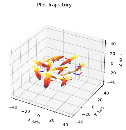
The final error should be many orders of magnitude smaller than the initial error, and the plot above should show landmarks close to a cube and poses close to a circular orbit -- confirming that Dogleg recovered the true reconstruction from a randomly perturbed start, using nothing but pixel observations, a single pose prior to fix the origin, and a single landmark prior to fix the scale.