Hybrid Data Association: Bayes Net and Bayes Tree

This short tutorial builds a one-scan data-association model for three objects with 2D positions, chooses a strong ordering, and solves the same hybrid posterior with sequential and multifrontal elimination.

import itertools

import gtsam
import numpy as np
import plotly.graph_objects as go
from gtsam.symbol_shorthand import A, X

1. Decision tree factor¶

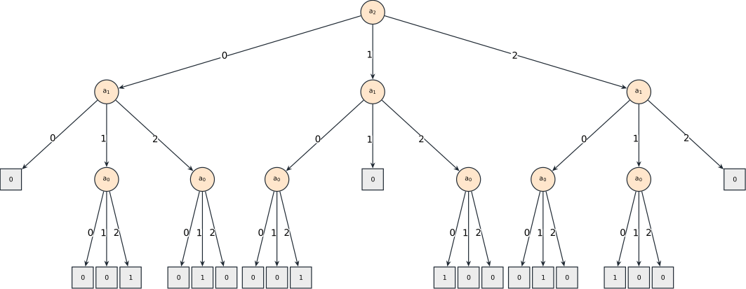
We first create the factor $c(a_0,a_1,a_2)$ drawn at the bottom of the factor graph. It is 1 when all three association variables have different values, and 0 otherwise.

GTSAM stores a DecisionTreeFactor as an algebraic decision tree. Each circular node branches on the value of one discrete variable, while each square leaf stores the resulting factor value. GTSAM puts the highest key at the root, so this tree starts with $a_2$ . A branch ends early when its value is already known: for example, $a_2=a_1$ immediately gives 0.

a = [(A(i), 3) for i in range(3)]

table = [
    float(len(set(association)) == 3)
    for association in itertools.product(range(3), repeat=3)
]
all_different = gtsam.DecisionTreeFactor(a, table)

print(type(all_different).__name__, "with", len(table), "table entries")

DecisionTreeFactor with 27 table entries

Decision tree for the all-different factor

2. Factor graph¶

The variables $x_i\in\mathbb R^2$ are object positions. Each variable $a_i\in\{0,1,2\}$ selects one measurement. The factors $p_i$ are Gaussian priors, $l_i$ are hybrid measurement likelihoods, and $c$ enforces that the three associations are all different.

predicted = np.array([[0.0, 0.0], [3.0, 0.0], [0.0, 3.0]])
measurements = np.array([[2.8, 0.2], [-0.1, 3.1], [0.2, -0.1]])
sigma = 1.5
prior_model = gtsam.noiseModel.Isotropic.Sigma(2, sigma)
measurement_model = gtsam.noiseModel.Isotropic.Sigma(2, sigma)

angles = np.linspace(0.0, 2.0 * np.pi, 80)
unit_circle = np.vstack((np.cos(angles), np.sin(angles)))
colors = ["#0072B2", "#E69F00", "#009E73"]

figure = go.Figure()
for i, (mean, color) in enumerate(zip(predicted, colors)):
    contour = mean[:, None] + sigma * unit_circle
    figure.add_trace(go.Scatter(
        x=contour[0], y=contour[1], mode="lines",
        line={"color": color}, legendgroup=f"x{i}", showlegend=False,
    ))
    figure.add_trace(go.Scatter(
        x=[mean[0]], y=[mean[1]], mode="markers+text", text=[f"x{i}"],
        textposition="bottom center", marker={"size": 12, "color": color},
        name=f"predicted x{i}", legendgroup=f"x{i}",
    ))

for m, (measurement, color) in enumerate(zip(measurements, colors)):
    contour = measurement[:, None] + sigma * unit_circle
    figure.add_trace(go.Scatter(
        x=contour[0], y=contour[1], mode="lines",
        line={"color": color, "dash": "dot"},
        legendgroup=f"z{m}", showlegend=False,
    ))
    figure.add_trace(go.Scatter(
        x=[measurement[0]], y=[measurement[1]], mode="markers+text",
        text=[f"z{m}"], textposition="top center",
        marker={"size": 13, "symbol": "x", "color": color},
        name=f"measurement z{m}", legendgroup=f"z{m}",
    ))

figure.update_layout(
    title="Predicted object positions and measurements",
    template="plotly_white", width=800, height=500,
    xaxis={"title": "x", "scaleanchor": "y", "scaleratio": 1},
    yaxis={"title": "y"}, legend={"orientation": "h", "y": -0.20},
    margin={"l": 50, "r": 20, "t": 60, "b": 90},
)
figure.show()

x = [X(i) for i in range(3)]
graph = gtsam.HybridGaussianFactorGraph()

for i in range(3):
    graph.push_back(gtsam.JacobianFactor(
        x[i], np.eye(2), predicted[i].reshape(2, 1), prior_model
    ))
    graph.push_back(gtsam.HybridGaussianFactor(a[i], [
        gtsam.JacobianFactor(
            x[i], np.eye(2), measurement.reshape(2, 1), measurement_model
        )
        for measurement in measurements
    ]))

graph.push_back(all_different)

print(type(graph).__name__, "with", graph.size(), "factors")

HybridGaussianFactorGraph with 7 factors

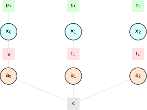
FGZ source: DataAssociationFactorGraph.fgz.

In the figure, cyan circles are the continuous position variables $x_i$ , and orange circles are the discrete association variables $a_i$ . Green squares are the Gaussian priors $p_i$ , red squares are the hybrid measurement likelihoods $l_i$ , and the gray square is the all-different factor $c$ .

3. Ordering¶

Hybrid elimination uses a strong ordering: eliminate all continuous positions before the discrete association variables.

ordering = gtsam.Ordering()
for key in x + [key for key, _ in a]:
    ordering.push_back(key)

print(ordering)

Position 0: x0, x1, x2, a0, a1, a2

4. Bayes net: create and optimize¶

Sequential elimination produces a HybridBayesNet. Its discrete part factors as $p(a_2)p(a_1\mid a_2)p(a_0\mid a_1,a_2)$ , and each continuous conditional is $p(x_i\mid a_i,Z)$ . optimize() selects the most probable integrated association and then optimizes the continuous variables conditioned on it.

bayes_net = graph.eliminateSequential(ordering)
net_result = bayes_net.optimize()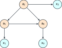

Hybrid Bayes net after sequential elimination

FGZ source: DataAssociationHybridBayesNet.fgz.

print(type(bayes_net).__name__, "with", bayes_net.size(), "conditionals")
print("association:", tuple(net_result.atDiscrete(A(i)) for i in range(3)))
for i in range(3):
    print(f"x{i}:", np.round(net_result.at(X(i)), 3))

HybridBayesNet with 6 conditionals
association: (2, 0, 1)
x0: [ 0.1  -0.05]
x1: [2.9 0.1]
x2: [-0.05  3.05]

5. Bayes tree: create and optimize¶

Multifrontal elimination represents the same posterior as a HybridBayesTree. Here its root is one discrete clique over $(a_0,a_1,a_2)$ , with three continuous child cliques. The two optimize() calls must agree. The Plotly chart shows the shared discrete posterior $p(A\mid Z)$ over the six legal associations.

bayes_tree = graph.eliminateMultifrontal(ordering)
tree_result = bayes_tree.optimize()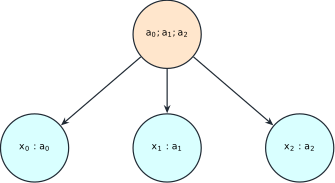

Hybrid Bayes tree after multifrontal elimination

FGZ source: DataAssociationHybridBayesTree.fgz.

print(type(bayes_tree).__name__, "with", bayes_tree.size(), "cliques")
print("association:", tuple(tree_result.atDiscrete(A(i)) for i in range(3)))
for i in range(3):
    print(f"x{i}:", np.round(tree_result.at(X(i)), 3))

HybridBayesTree with 4 cliques
association: (2, 0, 1)
x0: [ 0.1  -0.05]
x1: [2.9 0.1]
x2: [-0.05  3.05]

Below we show the probability distribution in the root clique.

associations = list(itertools.permutations(range(3)))
probabilities = []
discrete_posterior = bayes_net.discreteMarginal()
for association in associations:
    values = gtsam.DiscreteValues()
    for i, measurement in enumerate(association):
        values[A(i)] = measurement
    probabilities.append(discrete_posterior.evaluate(values))

figure = go.Figure(go.Bar(
    x=["".join(map(str, association)) for association in associations],
    y=probabilities,
    marker_color="#E69F00",
    text=[f"{probability:.3f}" for probability in probabilities],
    textposition="outside",
))
figure.update_layout(
    title="Association posterior p(A | Z)",
    template="plotly_white",
    width=720,
    height=420,
    xaxis_title="association (a0 a1 a2)",
    yaxis_title="probability",
    yaxis_range=[0, 1],
    showlegend=False,
)
figure.show()