GTSAM users typically solve pose-graph SLAM with a nonlinear optimizer initialized near the expected solution. That approach is fast and general, but its result can depend on the initial estimate because rotations make the problem nonconvex.
A certifiable approach rewrites supported factors as a quadratically constrained quadratic program (QCQP) and solves a convex semidefinite programming (SDP) relaxation. The SDP objective is a global lower bound on the QCQP objective. When the lifted SDP solution is numerically rank one, its recovered poses attain that bound and certify a globally optimal QCQP solution, up to numerical tolerance.
This example builds an anchored Pose3 ring, expresses its Frobenius factor graph exactly as a D=1 QCQP, solves monolithic and chordal SDP relaxations with MOSEK, and converts the recovered QCQP vectors to typed Pose3 values.
Related notebooks
Start with the QCQP example and QCQP API tutorial for the constrained optimization layer.
See the lifted SDP overview, monolithic SDP, and chordal SDP notebooks for the certifiable SDP APIs.
The Riemannian Staircase optimizer documents the Burer–Monteiro alternative.
The Rot2 and Rot3 rotation-averaging examples show the same certifiable pipeline without translation.

import numpy as np
import matplotlib.pyplot as plt
import gtsam
from gtsam.symbol_shorthand import X
Build an exact anchored ring
Frobenius factors compare homogeneous pose matrices, making their squared residuals quadratic in the matrix entries. This structure lets QcqpProblem translate the factor graph exactly into a D=1 QCQP.
A hard Frobenius prior fixes the global reference frame and removes gauge freedom. The relative measurements are mutually consistent around the cycle, so the QCQP admits a zero-cost solution at the ground-truth poses. This deliberately simple case makes the recovery and rank-one diagnostics easy to interpret.
# Generate five poses by repeatedly applying one spatial motion.
num_poses = 5
step = gtsam.Pose3(
    gtsam.Rot3.Rz(2.0 * np.pi / num_poses), np.array([2.0, 0.0, 0.0])
)
ground_truth = [gtsam.Pose3()]
for _ in range(1, num_poses):
    ground_truth.append(ground_truth[-1].compose(step))

# Anchor the global frame with a hard prior on the first pose matrix.
graph = gtsam.NonlinearFactorGraph()
graph.add(gtsam.FrobeniusPriorPose3(
    X(0), ground_truth[0].matrix(), gtsam.noiseModel.Constrained.All(16)
))

# Add exact relative-pose measurements, including the closing edge.
for i in range(num_poses):
    j = (i + 1) % num_poses
    graph.add(gtsam.FrobeniusBetweenFactorPose3(
        X(i), X(j), ground_truth[i].between(ground_truth[j]),
        gtsam.noiseModel.Isotropic.Sigma(6, 0.01),
    ))

# Convert the supported Frobenius factors into their exact QCQP form.
problem = gtsam.QcqpProblem(graph)
Solve both SDP formulations
The SDP relaxation replaces each rank-one outer product with a positive-semidefinite (PSD) matrix. The monolithic formulation collects the entire problem in one PSD cone. The chordal formulation uses the factor graph’s sparsity, a METIS ordering, and overlapping clique cones to represent the same relaxation more compactly.
After solve(), qcqpValues() independently recovers one homogeneous QCQP vector per pose. variableEVRs() returns the largest-to-second-largest eigenvalue ratio for each diagonal block; a large ratio indicates that the block is numerically rank one. The appropriate threshold depends on the application and solver tolerances.
# The SDP wrappers are present only in builds configured with MOSEK.
if not hasattr(gtsam, "MosekMonolithicSDP"):
    print("This GTSAM build does not include the optional MOSEK backend.")
    summaries = {}
else:
    # Solve the same QCQP using dense and sparsity-aware relaxations.
    solvers = {
        "monolithic": gtsam.MosekMonolithicSDP(problem),
        "chordal": gtsam.MosekChordalSDP(
            problem, gtsam.ChordalOrderingType.Metis
        ),
    }
    summaries = {}
    for name, solver in solvers.items():
        # A readable MOSEK solution is required before recovery queries.
        if not solver.solve({"intpntCoTolRelGap": 1e-10}):
            raise RuntimeError(f"{name} solve did not return a readable solution")

        # Recover homogeneous vectors, then decode them as typed Pose3 values.
        recovered = gtsam.extractQcqpValuesPose3(solver.qcqpValues())
        errors = np.array([
            np.linalg.norm(ground_truth[i].localCoordinates(recovered.atPose3(X(i))))
            for i in range(num_poses)
        ])

        # Retain accuracy, timing, and rank-one diagnostics for comparison.
        summaries[name] = {
            "objective": solver.objectiveValue(),
            "time": solver.solveTimeSeconds(),
            "errors": errors,
            "evrs": np.asarray(solver.variableEVRs()),
        }
        print(
            f"{name:10s} objective={solver.objectiveValue():.3e}, "
            f"max error={errors.max():.3e}, min EVR={summaries[name]['evrs'].min():.3e}"
        )
monolithic objective=3.201e-06, max error=5.034e-07, min EVR=1.517e+11
chordal objective=9.332e-08, max error=2.707e-08, min EVR=2.161e+12
# Compare the pose-wise recovery accuracy of the two formulations.
if summaries:
    indices = np.arange(num_poses)
    width = 0.36
    fig, axis = plt.subplots(figsize=(8, 4))
    axis.bar(
        indices - width / 2,
        summaries["monolithic"]["errors"],
        width,
        label="monolithic",
    )
    axis.bar(
        indices + width / 2,
        summaries["chordal"]["errors"],
        width,
        label="chordal",
    )
    axis.set(
        xlabel="pose index",
        ylabel="local-coordinate error norm",
        title="Recovered pose accuracy",
    )
    axis.set_yscale("log")
    axis.grid(axis="y", alpha=0.3)
    axis.legend()
    plt.tight_layout()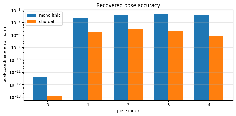
Reading the result
The objective should be near zero because every measurement is consistent with the anchored ground truth. The monolithic and chordal formulations should report nearly identical objectives and pose errors because they encode the same relaxation.
A large eigenvalue ratio indicates that a diagonal SDP block is effectively rank one, which supports recovering a single QCQP vector from it. Typed extraction then normalizes the homogeneous coordinate, projects the recovered rotation block to the nearest proper rotation, and retains the translation. If the eigenvalue ratios are not sufficiently large, users should treat the recovered poses as a heuristic rather than a certificate.